Does positive feedback necessarily mean runaway warming?
The skeptic argument...
Positive feedback means runaway warming
"One of the oft-cited predictions of potential warming is that a doubling of atmospheric carbon dioxide levels from pre-industrial levels — from 280 to 560 parts per million — would alone cause average global temperature to increase by about 1.2 °C. Recognizing the ho-hum nature of such a temperature change, the alarmist camp moved on to hypothesize that even this slight warming will cause irreversible changes in the atmosphere that, in turn, will cause more warming. These alleged "positive feedback" cycles supposedly will build upon each other to cause runaway global warming, according to the alarmists." (Junk Science)
What the science says...
| Select a level... |
Basic
|
Intermediate
|
Advanced
| ||||
| Positive feedback won't lead to runaway warming; diminishing returns on feedback cycles limit the amplification. | |||||||
Some skeptics ask, "If global warming has a positive feedback effect, then why don't we have runaway warming? The Earth has had high CO2 levels before: Why didn't it turn into an oven at that time?"
Positive feedback happens when the response to some change amplifies that change. For example: The Earth heats up, and some of the sea ice near the poles melts. Now bare water is exposed to the sun's rays, and absorbs more light than did the previous ice cover; so the planet heats up a little more.
Another mechanism for positive feedback: Atmospheric CO2 increases (due to burning of fossil fuels), so the enhanced greenhouse effect heats up the planet. The heating "bakes out" CO2 from the oceans and arctic tundras, so more CO2 is released.
In both of these cases, the "effect" reinforces the "cause", which will increase the "effect", which will reinforce the "cause"... So won't this spin out of control? The answer is, No, it will not, because each subsequent stage of reinforcement & increase will be weaker and weaker. The feedback cycles will go on and on, but there will be a diminishing of returns, so that after just a few cycles, it won't matter anymore.
The plot below shows how the temperature increases, when started off by an initial dollop of CO2, followed by many cycles of feedback. We've plotted this with three values of the strength of the feedback, and you can see that in each case, the temperature levels off after several rounds.
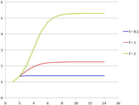
So the climatologists are not crazy to say that the positive feedback in the global-warming dynamic can lead to a factor of 3 in the final increase of temperature: That can be true, even though this feedback wasn't able to cook the Earth during previous periods of high CO2.
Note: A more detailed explanation is provided here.
Last updated on 13 September 2010 by nealjking.

Arguments


Basic
Intermediate
Advanced


If I may interject with an observation, I think you are very in danger of succumbing to hammer/nail syndrome ("when all you have is a hammer, every problem becomes a nail").
You are trying to view everything in terms of your own area of expertise, circuitry. While this is easier for you, it is going to lead you into trouble. Your analogies are fine for understanding a problem initially, but you will lose track of the fact that they are only analogies, and necessarily flawed.
To answer your questions and doubts I would very, very strongly suggest that you start by reading Spencer Weart's The Discovery of Global Warming -- A history. It's interesting, and you will learn a ton.
That being said, I'm surprised that I can't seem to find a transfer function based model of the climate. Its a control system, surely someone as formulated it as such. There is a well developed discipline called system identification which can derive transfer functions from auto-correlation of sampled data which would seem to be useful in this application.
That being said, there is no reason the differential equations that describe the climate can't be reformulated as a non-linear control system problem. Such a system should be able to describe in broad strokes the major features seen in the Paleo record. The problem is they don't. They can not explain how CO2 lags temperature through the entire cycle (and please don't point me to the CO2 lags thread. Been there. I want equations not hand waving about feedback).
Modelling is focused on representing the known physical system. A sweeping approach with simple equations doesnt tell us that much about what is really happening in the system. If you regard the "CO2 lags" as handwaving, then it because its not straightforward to put down a full physical model with coupled carbon-cycle model in a blog post. The point was explain, a/ considerable uncertainty remains in tying down CO2 feedbacks and b/ what we do know makes simplistic representation unlikely. These are the problems being tackled by AR5 models in paleoclimate. For details, go to the CMIP5 site and then look for ESM (Earth System Models).
I've never understood this objection. To me it has always seemed inescapable that, barring massive vulcanism or human injection of sequestered carbon into the atmosphere, simple cause and effect indicate that CO2 must lag temperature.
Seriously... how could CO2 levels rise prior to the temperature increase which causes this CO2 to be released from the oceans and frozen biological material? How could they fall prior to the cooling which allows the oceans to absorb more CO2 and sequesters organic carbon in ice?
Nor is the math required particularly complicated. The temperature swung by about 8 C during the glacial cycles. Offhand I don't know what the estimated factors are, but an 8 C swing could be produced from an orbital forcing of 0.8 C and total feedbacks (CO2, albedo, water vapor, et cetera) of f = 0.9;
0.8 C * [1/(1-0.9)] = 8 C
If we change the forcing in the equation above from 0.8 to 0 then the feedback effect would also be zero. Ergo, the CO2 temperature feedback MUST lag the orbital temperature forcing. Again, how is this anything but obvious?
How could CO2 lag temperature throughout the natural glaciation cycle? How could it NOT?
You asked for a formula showing how it could be possible that CO2 lags temperature throughout the glaciation cycle.
I provided an example.
In that example f was constant for simplicity. However, that does not mean I am claiming that f IS constant in the glaciation cycle... nor is f being constant a requirement for my example. Exactly the same conclusion would be reached with a value of f which changes over time... if the forcing effect is zero then, by definition, the feedback effect is zero - regardless of the value of f. Ergo, feedback MUST follow forcing.
Thus, whether f is constant or not is completely irrelevant to the issue at hand.
The simple forcing and feedback function in my prior message shows very clearly how a small forcing can produce a large change with a sufficiently large feedback factor. Exactly the same results could be achieved with an 'f' value which starts out at 0.95 and decreases down to 0.86 over time. Thus, we have a very simple mathematical model showing the possibility of CO2 (and other feedbacks) lagging temperature while still strongly influencing the total temperature change. This directly disproves your claim that CO2 must have "a negligible effect" if CO2 changes lag temperature changes.
A realistic model would require multiple feedback factors with different signs, different rates of change, and complex interrelation between the factors... basically a full scale climate model. However, that wasn't your stated request. You were asking how it was possible for CO2 to lag temperature... that question has been answered. Simple logic and mathematics both make it obvious that CO2 MUST lag temperature in the glaciation cycle.
The initial forcing is followed by an amplifying feedback, results continue to amplify (in decreasing amounts), a new stable state is reached (inter-glacial, for example). The initial forcing changes again, decreasing, allowing more CO2 to sequester in the oceans, hence another amplifying feedback until a new stable state is reached based upon the then current forcings (ice age). Rinse and repeat...
In the electronic analogies you have used, you need to incorporate resistor/capacitor or resistor/inductor elements - nothing is instantaneous in climate.
Now "non-linearity" handwaving is no better than feedback handwaving. But it seems to me that we should be putting more effort into understanding the nature of the limiting mechanisms. It just might save our bacon.
Seems to me you are looking for a level of difficulty found on Isaac Held's blog.
I really don't understand how people can have trouble with the CO2 lags stuff.
It's simple.
Increasing temperatures raise CO2 levels.
Raising CO2 levels raise temperatures.
Once something kicks the system up and raises temperatures initially (orbital forcings, for example), a feedback loop kicks in.
Without CO2, only the initial forcing takes effect, and temperatures rise only a little.
With CO2 (and other feedbacks), temperatures rise substantially further.
If you look at the ticker tape, it looks like temperatures are slowly rising and CO2 is following, but that is not what is happening.
What is happening is that temperature rose first as a result of a forcing, and then CO2 followed, pushing the temperature up, which pulled CO2 up, and so on.
This is really not that hard to understand, and there is no reason to express it in equations until you get the basic concept down.
It may well be that f(Co2,T,..) is such that this all makes sense. But it is not as intuitively obvious as the wand wavers would have us believe.
I no where claimed that CO2 must have a negligible effect on temperature nor do I believe that to be true. I stated that as the null hypothesis that can not be rejected on the basis of a just so story. Short of a mathematical proof, one must show how the data doesn't support the null hypothesis.
Wand wavers? Seriously? You are betraying quite a biased viewpoint there. This has been an interesting discussion, but that statement on your part indicates to me that you aren't very interested in answers.
Do you understand the original post in this thread? That indicates the positive feedback response (with the delays necessary in a physical system) leads to a finite amplification? And that this amplification applies for forcing deltas both upwards and downwards, amplifying the magnitude of those +/- forcings changes? And hence that any changes in forcing are amplified to larger changes in temperature via feedback?
Ice ages are initiated by decreasing insolation due to orbital mechanics. Interglacials are initiated by increasing insolation due (again) to orbital mechanics. Feedbacks turn a 1-3C forcing change into a 6-8C total change.
CO2 as a feedback won't rise to 'saturation', and I would consider that a strawman argument - nobody has said it would. I would have to consider that statement either misdirection or a severe lack of understanding on your part.
No, you're aren't approaching this with any bias...
Read the link Sphaerica provided - Spencer Weart's The Discovery of Global Warming -- A history. Based on the last 150+ years of physics, the radiative greenhouse effect and feedback via climate sensitivity are established science, poorly mapped electronics notwithstanding.
Yes and lags (or more probably time constants) have associated eigenvalues which in a system of at least 2nd order with positive feedback would generally produce spectral peaking, if the system is stable, and oscillation if it is not. The problem is there is no evidence of this peaking in the PSD of the paleo record which instead has all the characteristics of a highly regulated, dominate pole compensated control system (or alternatively a system phase-locked to transcendental forcing function). One explanation would be that the system poles are highly dissipative and so slight peaking is masked by noise (but the positive feedback should provide Q multiplication). There are other possible explanations (like the one in the above paper) which fit the data. We can't of course jump to conclusions but neither should we adhere to orthodoxy and close our minds to alternative hypotheses.
If you don't understand why the above is completely false, after having it explained to you several times, there really doesn't seem much point in continuing.
The temperature forcing from CO2 feedback is finite. There is no need to "overcome" an "ever increasing" temperature rise from CO2. The warming from CO2 stops... all on its own. After the orbital forcing which caused it does.
"Short of a mathematical proof, one must show how the data doesn't support the null hypothesis."
You do realize I (and others) already provided the mathematical proof, right?
CBDunkerson@70 "[condescending remarks deleted] The temperature forcing from CO2 feedback is finite. There is no need to "overcome" an "ever increasing" temperature rise from CO2. The warming from CO2 stops... all on its own. After the orbital forcing which caused it does."
See what I mean about inconsistency?
There is a common (though false) claim that the warming effect due to CO2 is currently saturated and that increasing atmospheric CO2 levels will thus cause no further warming. I'd assume that is what KR was referring to when he said that CO2 feedbacks would not rise to 'saturation'.
It is completely different from what I (and KR) said about temperature increases from CO2 being finite.
So no... there is no inconsistency. You just do not understand. Read it again. Really think about it. Ask specific questions.
As to people being 'condescending'... have you READ your own posts Mr. 'wand waving'?
jpat - the primary interest at the moment is how hot might it get in the next 100 years. The ice-age cycle is extremely interesting but carbon-cycle feedbacks are insignificant in that time period. We are providing all the CO2 at the moment, not nature. When the oceans start outgassing, it will get first. Also, low sensitivity is not supported by other evidence whereas 100ky problem has other solutions.
Its very important to recognise that climate theory is based on physics not paleoclimate. Paleoclimate studies can provide some constraints but primarily are useful as testing ground. Does our theory work in former times? The puzzles are paleoclimate arent challenges to theory - they are challenges of finding ways to constrain multiple theories which account for different forcings.
So to the question as to how hot could it get? Well paleoclimate does constrain that - as hot as the pliocene potentially.
CO2 solubility levels in the oceans are temperature dependent. Equations for the various sequestration pathways can be found in incredible detail in the Ocean acidification threads, but a 500-800 year lag time for a solubility response is supported by chemistry, ocean currents, and multiple observations.
My interpretation of 'saturation' in your previous post was that CO2 would continue to rise past the initial amplification due to it's own effects - which again contradicts finite amplification of a forcing. There is no inconsistency between CB's and my comments in that regard.
---
At this point it's unclear what your discussion is leading to. Climate is not a phase-locked oscillator, not an op-amp circuit. Your tone in this regard is rather remarkable - you seem to feel that because nobody has mapped the climate to your field of electronic circuitry that it's 'hand waving'.
Climate the response of the global energy distribution and hence chemical and hydrological responses due to multiple forcings, multiple deltas, with a fair number of positive and negative feedbacks adding up to a net positive amplification of ~3x, over which is laid non-linear interactions leading to chaotic variations (ENSO, weather).
Exact numbers for portions of this system have varying uncertainties, such as aerosol total effects, but the climate is surprisingly well understood as a boundary value driven physical system with chaotic variations.
Well, dontcha know, somebody has. It's dated (2001) and doesn't seem to have much about co2, so I don't know (and don't much care) if it's any good, but jpat might study the lecture series and report back.
Your comment contains a number of errors:Actually, "peak insolation" happens relatively quickly. That's the kick start. Insolation does not slowly increase to keep temperatures and CO2 rising. It increases relatively abruptly, and in so doing starts the rise in CO2 that drags temperatures further upward.No. dT/dt approaches a minimum as the effect of CO2 tapers off.This is wrong. First, the term "saturation" is ill-defined. I don't think you mean "so much we can't add anymore." What we care about is the temperature-effect of CO2, which is strongest when CO2 levels are low, and decreases as CO2 levels rise. After a while, adding more CO2 just doesn't affect temperatures all that much, so it doesn't add much more in the way of CO2. The feedback dies and a new, stable temperature is achieved.
This is because the temperature impact of CO2 is logarithmic, i.e. 1 unit of temperature change per doubling of CO2. So...
1x CO2 --> no change
2x CO2 --> 1 unit increase
4x CO2 --> 2 units increase
8x CO2 --> 3 units increase
and so on.No, as explained above. It contributes an ever decreasing forcing (otherwise you'd have a runaway effect).At the end of the interglacial, when orbital forcings change, there is a decrease in summer time insolation (both in strength and the length of the summer). This allows ice sheets to advance (or, more appropriately, keeps them from melting back to their starting point each summer). The advancing ice reflects rather than absorbs more and more incoming radiation. Temperatures drop correspondingly.
When temperatures drop, CO2 drops. When CO2 drops, temperatures drop. The entire cycle happens in reverse until much of the northern hemisphere is covered in ice.
You do realize that a mathematical proof excludes all other possibilities, right? Do you really think you've accomplished that?
Enter man. Add 115 ppm in just a hundred years (where the natural climb from 180 to 270 took thousands). This is a 0.5 fold increase. If we go all the way up to 540 ppm, double where we started, that is again another whole unit of temperature of increase.
Consider that the change from 180 to 270 is only a 0.5 fold increase in CO2. That's what pulls us out of a glacial period, over the course of thousands of years, and we have already today duplicated that forcing in a mere 100 years.
You are right in that the natural climate system had reached the point of diminishing returns. It was never going to push CO2 levels and temperatures above where they were at.
But that doesn't mean that CO2 will now somehow magically fail to have the same, predictable effect.
The plot below is what am using as a basis for my questions.
It is a sum-of-sines best fit to the adjusted vostok data where the period and amplitude of the forcing components was extracted by fourier analysis (and match near perfectly to the known Milkanovitch periods.) Since we can not know how the phase of each component is affected by the climate we adjust the phase of each component for best fit (r^2=.6).
Here's the Fourier analysis which was done with a technique called linear decomposition which avoids the spectral smearing one gets with windowing. The narrow line widths are strong indications that the forcings are astronomical as no natural terrestrial process could maintain this level of spectral purity over 500kYr.
Finally here's the same temperature extraction plotted with the CO2 extraction and scaled to equal amplitude for easy comparison.
In the first plot, note that the rapid decrease in temperature generally occurs near a dT/dt minima. In the last plot note that the CO2 is still rising at the temperature turn-around point.
I'm saying if one of my engineers brought me this plot and said that his system model indicated the red curve was the cause and the blue curve the effect I'd ask to see his equations :>) That's all I'm after here. No agenda, not trying to upset anyone or advocate a position. I just want to see the math for myself.
I think this has been pointed out several times, but there are more variables in the model.
KR and muoncounter - Thanks for the papers. Schwartz talks about some of the same taxonomical issues I tried to with my divider + VCVS analogy. I think incorporating something like this into the header on this topic would be helpful. In reading through the comments I see others have fallen into the same trap I did.
Speaking of math, did you verify that the time resolution of the Vostok core was sufficient to identify such a short period lag as your 'extracted astronomical signals' graph illustrates?
The question for feedback is that for a given delta-T, what are the changes in the feedback? For many the feedbacks, then this also depends on what current T is. Only water vapour is straightforward in this. Albedo depends on cloud response plus elevation versus freezing level.Methane is particularly complex, with multiple sources, some having temperature-triggered stores; and CO2 depends on your full carbon-cycle model.
Meissnet & Weaver
Calov et al
Matthews et al
At least examples of how complex the "equations" are. I'd say a lot more work is going to be done in this area though.
As you probably know, the Vostok data is not uniformly sampled. I resampled the data to a 5 year interval using standard interpolation and verified that the roll-off of the resampling was well above the signal band of interest. So yes, there's plenty of resolution.
jpat...some of the feedbacks are not easy to model realistically outside of an ESM (as they are called these days). For example, one paper scaddenp points to looks at vegetation feedbacks. These cannot spin out of control interminably as there is only so much land than can be converted to forest and back again. Soil carbon has similar constraints. Ocean chemisty, circulation and carbon sequestration is not nearly so straightforward a function of temp as you'd think. Martin hypothesized that dust delivery to the Southern Ocean can alter CO2 storage by stimulating Fe limited phytoplankton. That effect is constrained by availability of other nutrients, though, and would not scale proportionately with climate change.
Basically there are any number of ways to get an eventual damping of the CO2 -temp feedback. We're still trying to figure out which were really important.
When the forcing operates in the other direction, the now kilometres-thick ice sheets over North America and N Europe begin to melt, and can do so quite rapidly due to dynamical processes, especially when the height of the ice sheet begins to drop. That aids all the other feedbacks operating in a warming direction, but there is an element of self-limiting as eventually the big ice sheets have shrunk and so the albedo component can't drop quite so fast, and the forcing is no longer at a maximum. In order to continue the melting into the next vulnerable ice sheets - Greenland and West antarctica - you need an extra forcing kick.
CO2 can operate as a forcing or a feedback (the molecules have no memory of how they got into the atmosphere, they just trap heat), and by releasing lots of CO2, we've provided the extra kick in forcing, which means that Arctic sea ice, Greenland and West Antarctica are vulnerable. There's nothing magical about why most interglacials appear to have approximately similar magnitudes, as that is a function of continental configuration and the length of the forcing. During the last interglacial, it's likely that parts of Greenland and West Antarctica melted as well.
That's a very long way of saying that you cannot easily represent the full interrelationships of forcings and feedbacks with a simple function. In fact, the best way to capture the relationship is to build a model of all the relationships (a simple function is merely a simple model after all), incorporating all the radiative physics as best we can. You'll get even better results if your model is a spatial one that can capture trickier concepts like continental configurations and ocean circulations. This has been done, they are called GCMs.
You didn't seriously think that the experts in this field who have worked on this for their whole careers hadn't thought of all this? You can't come at climate science from an unrelated field and completely grasp all the complexities without a great deal of effort. You seemed to be suggesting that you can, if your misconceptions about the palaeo record & CO2 and how much it's all 'figured out' in #58 and elsewhere are anything to go by. I can only recommend you re-read Sphaerica's advice in #51.
Forcing function F drives the input. It gets summed with the feedback signal and converted to temperature by Gain2. The feed back path encapsulates the functional relationship between Co2 and temperature. The transfer function models the time lag between a change in temperature and the corresponding change in CO2 concentration at node C. Gain1 handles the conversion from CO2 to radiant energy. The feedback is positive but low enough that the system is stable.
The paleo temperature record corresponds to the signal at T, the CO2 record to the signal at C. We ask ourselves, what is the expected time relation between T and C under closed loop conditions? Answer: Same as under open loop conditions! I.e. feedback can not change the open-loop relationship between T and C. If the physical mechanism that produces CO2 when the temperature rises includes a lag (and it does), we expect to see that same lag under closed loop conditions. How can it be otherwise? The relationship between T and C is defined by the blocks between them. And note that relationship is completely independent of the complexity of the transfer function which could include other internal feedback loops, other gain paths etc.
I can think of no system formulation that could possible convert a lagging signal to a leading signal. I hope this clears up my conundrum.
[DB] Since you are fond of analogies, let me share this one with you:
Your conundrum, distilled, is that you are treating climate science as some that learn a foreign language: you are insisting upon translating the words you hear into English before assembling them into sentences. However, to truly learn a foreign language, one must learn enough vocabulary, sentence structure and syntax to understand the foreign language in your head without the need for translation. In essence, you need to be able to think in that foreign language before true understanding of it is then reached.
That is what is retarding your understanding. As it has retarded the understanding of electrical engineer-types like RW1 and co2isnotevil before you.
In your electical system above, it gets there via the slow feedback, and so there would be a delay between the temperature change (which has to rise first) and the CO2 (which amplifies the temperature change, but rises later).
Now consider what happens if you release a very large amount of CO2 directly into the atmosphere. We've done that, adding more that the entire CO2 difference between LGM and Holocene within about 100 years. Does the CO2 wait patiently for 800 years before operating? No, it starts working as soon as a suitable packet of longwave radiation passes by! How will your graph look now? Will there be much of a lag between temperature response and CO2? Which one will rise first, all other factors excluded?
Second, can you build one so that feedback response is different when temperature is rising than when it is falling?
You are currently paralyzed by (a) restricting your thinking to circuit design and (b) trying to oversimplify the system.
In particular, you need multiple feedback loops (short term CO2, long term CO2, H2O, low equatorial clouds, low NH clouds, high clouds, ice, CH4, etc.) which all interact with each other, some in non-linear ways, and with clock cycles that introduce varying delays. They are also bounded in unexpected ways. For example, the extent of ice cover can only advance and retreat so far, and ice further south is much more powerful since it covers a larger area, winter daylight hours are longer, and the sun strikes at a stronger angle of incidence.
So the forcing-feedback effect Fice of the retreat of ice ∆I in response to a positive temperature change ∆T is also dependent on the actual ice extent I at the time of the change combined with the orbital configuration Xorbit. The ice extent I is itself dependent not only on temperature but also the current orbital configuration Xorbit. Fice is also moderated by the amount of low NH clouds Clow NH and aerosols A (since both of these block light and thereby negate any effects of ice on the surface).
That's just a simplified set up for ice. The effects of CO2 and H2O are similarly complexly moderated (ice, aerosols and low clouds reflect visible light, resulting in less IR to feed the greenhouse effect, for example).
The feedback loop for H2O is far, far faster than that for CO2. The different mechanisms for changing CO2 in the atmosphere (vegetation growth, vegetation decay, temperature-dependent ocean absorption/out-gassing, the very important biological pump, etc.) all work at different rates. In addition, the growth and decay of vegetation, like ice, is dependent on latitude... lower latitudes have more area, and are more hospitable to plant growth, so the initial effects of the retreat of the ice sheets on CO2 changes related to vegetation are far greater at lower latitudes than later retreat further north.
The biological pump which is thought to cause the most abrupt and important changes in atmospheric CO2 in transitions between glacials and interglacials is, like all other factors in the system, bounded, non-linear and self-limiting.
The entire system is just far, far, far more complicated than you are considering right now. A mechanic who tries to model the system in terms of an accelerator pedal, fuel line, fuel pump, etc. would have a better chance of producing an accurate analog of the system than an electrical engineer.
I said it before: hammer/nail syndrome
You are very strongly advised to stop trying to translate everything into your chosen profession and perspective, and instead to learn the science as it stands. You will be eternally stalled if you keep trying to hammer 27 round climate pegs into one, square EE hole.
You should also consider that heat is not distributed evenly across the planet. A mean global temperature change of ∆T may be conceptually divided into at least 7 separate values by latitude (although the actual system is continuous in nature): equatorial, and NH and SH values for sub-tropical, temperate, and polar. These changes are non-linear (for instance, warming now is much greater at the equator than the south pole, and much greater at the north pole than the equator.
As already explained, the strength of the effects of such temperature changes on feedback factors (ice, vegetation, ocean dynamics) vary by latitude as well, so now for each latitude you have a different ∆T, a different area, a different potential for impact (due to area, amount of insolation, and angle of incidence of the sun) and so an entirely different feedback value dependent upon absolute temperature and latitude.