


 Arguments


Watts' New Paper - Analysis and Critique
Posted on 2 August 2012 by dana1981, Kevin C
"An area and distance weighted analysis of the impacts of station exposure on the U.S. Historical Climatology Network temperatures and temperature trends"
Paper authors: A. Watts, E. Jones, S. McIntyre and E. R. Christy
In an unpublished paper, Watts et al. raise new questions about the adjustments applied to the U.S. Historical Climatology Network (USHCN) station data (which also form part of the GHCN global dataset). Ultimately the paper concludes "that reported 1979-2008 U.S. temperature trends are spuriously doubled." However, this conclusion is not supported by the analysis in the paper itself. Here we offer preliminary constructive criticism, noting some issues we have identified with the paper in its current form, which we suggest the authors address prior to submittal to a journal. As it currently stands, the issues we discuss below appear to entirely compromise the conclusions of the paper.
The Underlying Problem
In reaching the conclusion that the adjustments applied to the USHCN data spuriously double the actual trend, the authors rely on the difference between the NCDC homogenised data (adjusted to remove non-climate influences, discussed in detail below) and the raw data as calculated by Watts et al. The conclusion therefore relies on an assumption that the NCDC adjustments are not physically warranted. They do not demonstrate this in the paper. They also do not demonstrate that their own ‘raw’ trends are homogeneous.
Ultimately Watts et al. fail to account for changing time of observations, that instruments change, or that weather stations are sometimes relocated, causing them to wrongly conclude that uncorrected data are much better than data that takes all this into account.
Changing Time of Observations
The purpose of the paper is to determine whether artificial heat sources have biased the USHCN data. However, accounting for urban heat sources is not the only adjustment which must be made to the raw temperature data. Accounting for the time of observations (TOB), for example, is a major adjustment which must be made to the raw data (i.e. see Schaal et al. 1977 and Karl et al. 1986).
For example, if observations are taken and maximum-minimum thermometers reset in the early morning, near the time of minimum temperature, a particularly cold night may be double-counted, once for the preceding day and once for the current day. Conversely, with afternoon observations, particularly hot days will be counted twice for the same reason. Hence, maximum and minimum temperatures measured for a day ending in the afternoon tend to be warmer on average than those measured for a day ending in the early morning, with the size of the difference varying from place to place.
Unlike most countries, the United States does not have a standard observation time for most of its observing network. There has been a systematic tendency over time for American stations to shift from evening to morning observations, resulting in an artificial cooling of temperature data at the stations affected, as noted by Karl et al. 1986. In a lecture, Karl noted:
"There is practically no time of observation bias in urban-based stations which have taken their measurements punctually always at the same time, while in the rural stations the times of observation have changed. The change has usually happened from the afternoon to the morning. This causes a cooling bias in the data of the rural stations. Therefore one must correct for the time of observation bias before one tries to determine the effect of the urban heat island"
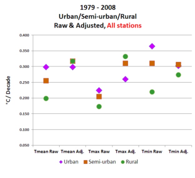
Note in Watts Figure 16, by far the largest adjustments (in the warming direction) are for rural stations, which is to be expected if TOB is introducing a cool bias at those stations, as Karl discusses.
Instruments Change, Stations Move
As Zeke Hausfather has also discussed, the biggest network-wide inhomogeneity in the US record is due to the systematic shift from manually-read liquid-in-glass thermometers placed in a louvred screen (referred to in the U.S. as a Cotton Region Shelter and elsewhere as a Stevenson screen) to automated probes (MMTS) in cylindrical plastic shelters across large parts of the network in the mid- to late-1980s. This widespread equipment change caused an artificial cooling in the record due to differences in the behaviour of the sensors and the sheltering of the instruments. This is discussed in a number of papers, for example Menne et al. 2009 and 2010, and like TOB does not appear to be accounted for by Watts et al.
Additionally, the Watts paper does not show how or whether the raw data were adjusted to account for issues such as sites closing or moving from one location to another. The movement of a site to a location with a slightly different mean climatology will also result in spurious changes to the data. The Watts paper provides no details as to how or whether this was accounted for, or how the raw data were anomalised.
Quite simply, the data are homogenised for a reason. Watts et al. are making the case that the raw data are a ‘ground truth’ against which the homogenisations should be judged. Not only is this unsupported in the literature, the results in this paper do nothing to demonstrate that. It is simply wrong to assume that all the trends in raw data are correct, or that differences between raw and adjusted data are solely due to urban heat influences. However, these wrong assumptions are the basis of the Watts conclusion regarding the 'spurious doubling' of the warming trend.
The Amplification Factor
The conclusion regarding the lower surface temperature warming trend is also at odds with the satellite temperature data. Over the continental USA (CONUS), satellites show a 0.24°C per decade warming trend over the timeframe in question. According to Klotzbach et al. (2010), which the Watts paper references, there should be an amplification factor of ~1.1 between surface and lower troposphere temperatures over land (greater atmospheric warming having to do with water vapor amplification). Thus if the satellite measurements were correct, we would expect to see a surface temperature trend of close to 0.22°C per decade for the CONUS; instead, the Watts paper claims the trend is much lower at 0.155°C per decade.
This suggests that either the satellites are biased high, which is rather implausible (i.e. see Mears et al. 2011 which suggests they are biased low), or the Watts results are biased low. The Watts paper tries to explain the discrepancy by claiming that the amplification factor over land ranges from 1.1 to 1.4 in various climate models, but does not provide a source to support this claim, which does not appear to be correct (this may be a reasonable range for global amplification factors, but not for land-only).
A discussion between Gavin Schmidt and Steve McIntyre on this subject led to the conclusion that the land-only amplification factor falls in the range of 0.78 to 1.23 (average over all global land areas), with a model mean close to 1 (using a script developed by McIntyre on 24 different models). Note that McIntyre is a co-author of Watts et al., but has only helped with the statistical analysis and did not comment on the whole paper before Watts made it public. We suggest that he share his land-only amplification factor discussion with his co-authors.
Another important consideration is that the amplification factor also varies by latitude. For example Vinnikov et al. (2005) found that at the CONUS latitude (approximately 40°, on average), models predict an amplification factor of approximately 1 (see their Figure 9). Note that this is the amplification factor over both land and ocean at this latitude. Since the amplification factor over land is less than that over the oceans, this suggests that the amplification factor over the CONUS land may even be less than 1.
Combining the latitude and land-only status of the CONUS, the amplification factor may very well be less than 1, but a range of values significantly lower than the 1.1 to 1.4 range used in the Watts paper would be reasonable.
Note also that as discussed above, the satellite data (like all data) are imperfect and are not a 'gold standard'. They are a useful tool for comparison in this study, but the satellite trends should not be assumed to be perfect measurements.
More Apples and Oranges
Watts et al. compare the best sited Class 1 and 2 stations (using their categorisation) to the total homogenised network. Strictly speaking, this is comparing apples and oranges; Watts' data are an inhomogeneous sub-sample of the network compared to a homogeneous total network. In practice, this methodological error doesn’t make much difference, since the homogenisation applied by NCDC produces uniform trends in all of the various classes.
However the use of a smaller network has disadvantages. When taking a gridded average of a sparse network, the impact of inhomogeneities is likely amplified and the overall uncertainty of variability and change in the timeseries increases.
The Class 1 & 2 sites used by Watts in this context represent just 20% of all the total CONUS network. The comparison of the raw Class 1 & 2 sites with the same network of homogenised data in Watts' own Figure 18 indicates likely inhomogeneities in that raw data. Watts et al. argue that the raw and adjusted Class 1 & 2 trends in Figures 18a and 18b are so different because "well sited stations are adjusted upward to match the already-adjusted poor stations," but this is simply not how the homogenization process is done. In reality the difference is likely due to the biases we have discussed above, indicating that the Watts raw data is inhomogeneous and influenced by these non-climate effects.
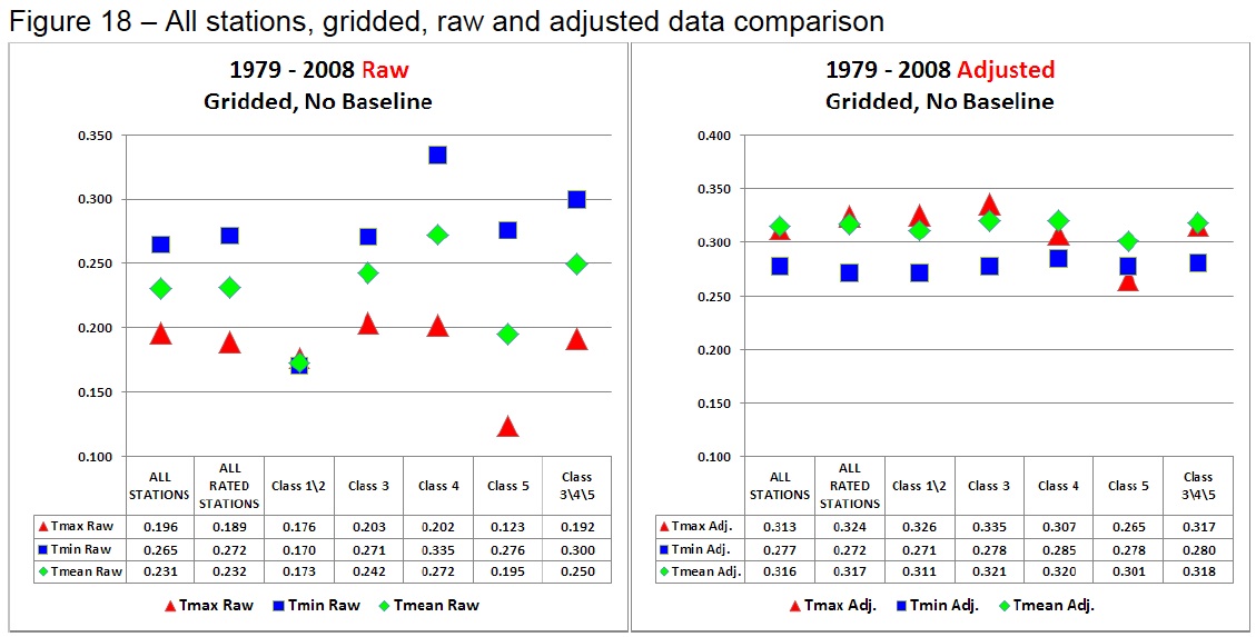
Determining whether or not the Class 1 & 2 raw data is homogeneous is therefore a key requirement of a revised manuscript. And since the Class 1 & 2 sites have been selected for good exposure, Watts et al. would need to show the cause of any statistical discontinuities that they find. This work has already been done by NCDC in the Menne at al. papers, which show influences from the range of factors discussed above, and not just urban influence.
The Watts final conclusion that adjusted temperature trends are 'spuriously doubled' (0.155°C vs. 0.309°C per decade raw vs. adjusted data) relies on a simple assumption — that the raw data must be correct and the homogenised data incorrect. There is no a priori basis for this assumption and it is unsupported by the literature.
Adjustments Make Little Difference Globally
While Watts et al. identify possible issues concerning the adjustments applied to station temperature records, it wisely makes no attempt to assess the global impact of the adjustments, which are beyond the scope of the work. Nonetheless, this is a significant question from a public interest perspective.
In order to answer this question, we willl try and estimate the maximum possible impact of station adjustments on the instrumental temperature record. To minimise the warming signal, we will use the simplest method for calculating a global temperature average - the CRU method, which is known to yield poor coverage at high latitudes and hence underestimate recent warming. Further, we'll assume that entirety of the data adjustments are wrong (ignoring proven bias corrections such as TOB). If we calculate land temperature averages from both the raw and adjusted data, we can see how much difference the adjustments make. The result is shown in the figure below (red and green lines).

Just to be absolutely sure, we can do a further calculation using just rural unadjusted data (using the GHCN station classifications) - the blue line.
While the adjustments do make a difference, the difference is small compared to the overall warming signal since 1979. Using a more sophisticated temperature calculation reduces this difference. Furthermore, we are only looking at land temperatures - 30% of the planet. Including the remaining 70% of the planet (the oceans which, if not precisely rural, are certainly not urban!) dramatically reduces the remaining impact of the GHCN adjustments. Indeed, comparison of warming trends over the oceans and over large inland lakes (including the North American Great Lakes) shows a high degree of consistency with terrestrial trends. Warming over the oceans and lakes is presumably not due to urbanisation.
The entire CRU-type calculation requires 65 lines of python code (by comparison, a modern airliner requires upwards of a million lines of code to fly). The code is available below.
Show code
Many others have done this comparison, including Caerbannog and Zeke Hausfather. Fawcett et al (2012) provide a comprehensive assessment of the sensitivity of Australian temperature trends to network and homogenisation choices, including comparison with an unhomogenised gridded analysis of Australian temperatures. Furthermore, the BEST project has obtained a similar result with a different, independent implementation of the station homogenization algorithm. It would be surprising if an independent approach were to yield a similar but incorrect result by chance.
Do the overall adjustments make a difference? Yes. Are they justified? Yes, according to the body of scientific literature. Watts raises a scientific issue, but one which only affects part of the adjustment. Does it matter? Not very much. Even if the entirety of the adjustments were wrong, we still see unprecedented warming over the past 40 years. And there is certainly not a factor of two difference between global warming trends in the raw and adjusted data.
Constructive Criticisms
It's worth noting that Peter Thorne of NCDC was interviewed by Andrew Revkin, and discussed three papers which NCDC has recently published (see here, here, here). In the first of those linked papers, they actually concluded that there likely remains a residual cool bias in the adjusted data, and that the adjusted data are consistent with reanalysis data (detailed in the third linked paper). Watts et al. do not address these papers. Ironically Watts responded to that interview by saying that Thorne needs to get out into the real world, but it is Watts et al. who have not accounted for real world effects like TOB, station movement, instrument changes, etc.
In its current form, the Watts paper contains little in the way of useful analysis. There are too many potential sources of bias which are not accounted for, too many apples-to-oranges comparisons, and they cannot draw any conclusions about urban heat influences until their data are homogenized and other non-climate influences are removed.
The primary conclusion of the paper, aside from not being supported by the analysis, is simply implausible. The CONUS surface warming trend proposed by the Watts paper appears to be inconsistent with the satellite observations, and overall global trends in raw data do not differ dramatically from those in the adjusted data. Comparing raw to adjusted data globally shows a rather small difference in long-term trends; far smaller than a factor of two.
The flaws we have identified entirely compromise the conclusions of the paper. Ultimately Watts et al. assume that all adjustments are 'spurious' unless due to urban heat influences, when in fact most of their identified discrepancy likely boils down to important adjustments for instrumental changes, TOB, and other influences they have not accounted for in their analysis. Watts et al. attempt to justify their assumption by asserting "well sited stations are adjusted upward to match the already-adjusted poor stations," but this is simply not how the homogenization process is done.
Fortunately McIntyre has acknowledged that TOB must be considered in their analysis, as has Watts, which is a good start, but they must also account for the other biases noted above in order to draw any valid conclusions about urban heat influences.
In conclusion, Watts et al. of course deserve the right to try to make their case in the peer-reviewed literature, however implausible that case appears to be. Therefore, we hope they will consider addressing the important concerns detailed above before they submit the paper to a journal. Otherwise we suspect the paper will not fare well in the peer review process. With said caveats carefully addressed and the conclusions amended if and where necessary, the paper has the potential to be a useful contribution to the climate science literature.


youone would even refer to a just submitted paper with the year of publication attached to it. I think the normal nomenclature would be to refer to it as "Watts et al, submitted."Continuing from an unfinished page here:
As I pointed out on a WUWT thread that claimed adjustments were distorting the data,
Various replies (arguments from authority, etc) followed, mostly ignoring the rather copious literature on time of observation bias.
You'll be seeing the real thing soon enough. It has been a long hard slog with many corrections.
Here we offer preliminary constructive criticism, noting some issues we have identified with the paper in its current form, which we suggest the authors address prior to submittal to a journal.
We appreiate the criticisms here. Some of them are quite valid. We will be providing answers on the homogenization issue. TOBS, station moves, and MMTS conversion are now fully addressed. Data is fully anomalized (though we show both sets).
We will, of course, provide documentation showing all comparison. For example, you can compare Class 1\2 stations raw (+MMTS adjustment) with fully adjusted Class 1\2 data (or with any other set or subset, either raw+MMTS or fully adjusted.
If anyone has any questions at this point, i will be happy to answer them.
I'd posit that someone here, who may have some conection to Anthony, invite him to *politely* discuss Dana and Kevin's analysis, in the SkS spirit.
That'll be me. Fire away.
Evan @67... That suggestion for a discussion was made almost two years ago (and made by a commenter, not the original authors of the article). It seems prudent to wait until the paper is actually published and then SkS authors will review the paper again.
Rob Honeycutt @68.
The appearance of an ebullient Evan Jones to claim (in the present tense) credit for (actually) an almost three-year-old comment may be down to a new outlet appearing for the publication of atmospheric science. It is called The Open Atmospheric Society and according to this web-page the founder is a chap called Anthony Willard Watts which should make papers written by Anthony Willard Watts a lot easier to get published.
http://theoas.org/
http://dailycaller.com/2015/06/19/skeptics-found-scientific-society-to-escape-journals-that-keep-out-dissenters/
MA Rogers... A tad ironic being that one of the latest conspiracy theories about Cook13 is that Environmental Research Letters was created for the purpose of publishing the 97% Consensus paper.
Rob Honeycutt - An excellent, and very amusing, point.
Oh, and you're right. It was three years ago, not two! Amazing.
For me, closer to four. I have been at it since Fall et al. (2011), of which I was a co-author. It was necessary to convert the ratings from Leroy (1999) to Leroy (2012). After the criticisms here and elsewhere, it was then necessary to address the outstanding issue of TOBS, station moves, and MMTS conversion. Then swing it all over from USHCN2.0 to USHCN 2.5.
The appearance of an ebullient Evan Jones to claim (in the present tense) credit for (actually) an almost three-year-old comment
Anthony made the decision to pre-release in order to obtain hostile independent review so any issues could be addressed before submission. Having done that, peer review will go a lot easier.
I hashed this out on Stoat, but we made note of the criticisms here, as well. I am not disputing the problems with raw data. But I do have some issues with the adjustment procedure, especially with homogenization.
Doc. VV and I burned through a forum-plus on Sou's blog discussing that point. He says aour findings are interesting, but thinks the divergence between the well and poorly sited stations will be acounted for by jumps. But I've run the graphs, and the divergence is as smooth as silk. He also points out that homogenization will not work if thereis a systematic error in the data. In this cas, that systematic error is microsite.
The problem is that only 22% of sample is well sited, so the well sited stations are brought into line with the poorly sited stations rather than the other way around. If one does not address siting, it is a very easy error to miss. I find it is quite unintentional on NOAA's part, but it is a severe error, nonetheless.
If anyone has any specific questions about the current state of the study, I will be pleased to answer.
@Evan Jones: Is this the "game-changing" paper that Watts promised a few years ago?
Evan Jones - The only relevant 'systematic error' would of course be one in trends, in change. The issue of site quality is relevant to certainty bounds, but unless you have evidence of consistent trends in microsite driven changes in temperatures, I don't think there's much support for overall missed trend errors.
Not to mention that the US is only ~4% of the globe. I am always saddened by the arguments (both implicit and explicit) on WUWT and other sites claiming (without evidence, mind you) that US adjustments are wrong, usually with claims of malicious distortion and conspiracies, and therefore that global temperature trend estimates are also claimed to be wholly wrong.
I fully expect that the upcoming paper, regardless of the strengths or weaknesses of the work and data, will be be (mis)used as part of such arguments, just as Fall et al 2011 was. Which IMO is unfortunate; it subtracts from the actual worth of these papers.
John Hartz... Yup, that's the one. Which brings up a good point.
If Watts had "[decided] to pre-release in order to obtain hostile independent review" why would he be touting it as a "game changing paper?" I find this notion to be dubious at best and downright deceptive if true.
If you have a paper where you're looking for independent public review, then you should state as much up front! That's not what Tony did. He posted it making wildly unsubstantiated claims about it being something important, influential and about to be published. It strikes me as being supremely self-deluded to suggest posting it before publication was for the purposes of review.
Rob Honeycutt @76.
Indeed, for all the world, the description of the pre-release at the time was not consistent with the suggestion @73 that it was a "pre-release in order to obtain hostile independent review so any issues could be addressed before submission," and certainly never a review which would last for years. Planet Wattsupia was actually shut down to allow Watts to get the paper finished and rushed out into the public domain. The official "Backstory" to this drama ended thus:-
(*Kenji is a dog, apparently.) So would anyone in their right mind describe the hammering the paper has received since the press release as a "final polish"?
Rob Honeycutt:
If I were authoring a "game changing" paper on manmade climate change, I certainly would concentrate on completing it as expeditiously as possible .
It appears that Watts has been too busy throwing red meat to his WUWT followers to have focused on his "game changer."
What a farce!
Evan Jones,
You are claiming major changes have been made. You ask for feedback, but you have not shown what the major changes are. How do you expect us to make comments when you do not show your changes? If you want additional feedback, it is your responsibility to show the changes you have made so that people here can evaluate them. So far you are just advertising your "new" paper.
Now now, folks. Watts, Jones, etc. can hold Fall et al 2011 to their credit, as a paper that took considerable work and was published in a peer reviewed journal - despite the conclusions going against their expectations:
While the initial unpublished and apparently unreviewed paper received a rough reception in its previous foray, due in large part to really significant issues regarding incorrect conclusions drawn by not applying any of the significant known corrections for data errors, I for one am willing to withhold judgement on the next iteration until after I've read it.
Mind you, I do not hold high expectations, considering the quality (or lack thereof) of error correction and homogenization discussions that have occurred at WUWT. But we'll have to wait and see.
Is this the "game-changing" paper that Watts promised a few years ago?
Yes.
The only relevant 'systematic error' would of course be one in trends, in change.
Yes, of course.
The issue of site quality is relevant to certainty bounds, but unless you have evidence of consistent trends in microsite driven changes in temperatures, I don't think there's much support for overall missed trend errors.
I agree completely. We have powerful evidence of the effect on trend (sic).
Not to mention that the US is only ~4% of the globe.
Not relevant in this particular case. All that is required is a sufficient amount of data to compare siting. What's sauce for the USHCN is sace for the GHCN. But I also agree that a survey of all GHCN stations is called for. But that's not so easy (if even possible at this time) for a whole host of reasons.
I am always saddened by the arguments (both implicit and explicit) on WUWT and other sites claiming (without evidence, mind you) that US adjustments are wrong, usually with claims of malicious distortion and conspiracies, and therefore that global temperature trend estimates are also claimed to be wholly wrong.
I claim all that — with very strong evidence — but WITHOUT the conspiracy theories. I do not think this is fraud, merely an error. An understandable one, one I might easily have made myself.
All data and methods will be fully archived in a form that can be easily altered or re-binned if you think we got parts of it wrong, so you can run your own versions should you desire. I will assist. Bear in mind that we are not trying to convince our "pals". That's always easy. Too easy. We are trying to convince our opponents in this.
I fully expect that the upcoming paper, regardless of the strengths or weaknesses of the work and data, will be be (mis)used as part of such arguments, just as Fall et al 2011 was. Which IMO is unfortunate; it subtracts from the actual worth of these papers.
I have and will continue to insist publicly that the results of these papers do not dispute the reality of AGW. But it does dispute the amount.
If you have a paper where you're looking for independent public review, then you should state as much up front! That's not what Tony did. He posted it making wildly unsubstantiated claims about it being something important, influential and about to be published. It strikes me as being supremely self-deluded to suggest posting it before publication was for the purposes of review.
But we did.
The pre-release of this paper follows the practice embraced by Dr. Richard Muller, of the Berkeley Earth Surface Temperature project in a June 2011 interview with Scientific American’s Michael Lemonick in “Science Talk”, said:
I know that is prior to acceptance, but in the tradition that I grew up in (under Nobel Laureate Luis Alvarez) we always widely distributed “preprints” of papers prior to their publication or even submission. That guaranteed a much wider peer review than we obtained from mere referees.
That is exactly what our "purposes" were, and that is exactly what we did. And I have been addressing the resulting (exraordinarily valuable) independent review ever since. It takes time.
If I were authoring a "game changing" paper on manmade climate change, I certainly would concentrate on completing it as expeditiously as possible .
It appears that Watts has been too busy throwing red meat to his WUWT followers to have focused on his "game changer."
What a farce!
He has had to wait on me. Sorry about that.And I have been concentrating on completing it. I have put in ~3000 hours on this since Fall et al., give or take, plus fulltime work. It has consumed my life. And now, finally, we are just about "there".
You are claiming major changes have been made. You ask for feedback, but you have not shown what the major changes are.
Fair enough. I will go into some detail. The three major issues are addressed:
1.) MMTS Adjustment: All MMTS station data is jumped at (and after) the month of conversion according to Menne (2009) data: Tmax: +0.10C, Tmin: -0.025C, Tmean: +0.0375C. (There is also an issue with CRS, per se., which I'll discuss if you wish.)
2.) TOBS: Stations with TOBS flips from afternoon to morning (and a small handful vice-versa) are dropped. This avoids the issue of TOBS adjustment while still maintaining a robust sample.
3.) Station Moves: Any station that has been moved after Apr. 1980 is dropped unless both locations are known AND the rating remains the same. Also, if the rating changed during the study period (1979 - 2008), we dropped the station even if the location(s) was known. It is not controversial that a change in site rating will likely affect trend (by creating a jump). But what we want to demonstrate, unequivocally, is that trends (either warming or cooling) are exaggerated by poor microsite even if the microsite rating is unchanged throughout the study period.
4.) In addition, we provide data during the cooling interval from 1999-2008. A ten-year period is obviously not sufficient to assess overall climate change (and we are not trying to do that). But it is quite sufficient to demonstrate that during that period that the badly sited stations cooled more quickly than the well sited stations.
Heat Sink Effect works both ways. It exaggerates trend in either direction, warming or cooling. What goes up must come down. The only reason that poor microsite has exaggerated warming is that there has been real, genuine warming to exaggerate in the first place.
Our hypothesis does not dispute global warming — it requires it.
Note: After dropping stations as per the above, we are left with a sample of 410 unperturbed stations (both well and poorly sited). However, we are not cherrypicking: the sataions we dropped have substantially cooler trends than the ones we retained.
Evan Jones:
Since you are doing all of the heavy lifting on this paper, why is Watts listed as the lead author?
Now now, folks.
THANK you for that. Yes, we did not withhold our findings even though they disputed our hypothesis. One of the casrdinal rules of science is that one must never withhold one's findings.
I apprecite that you withhold judgment untill you have an opportunity to read the new version of the paper and carefully examine the supporting data.
We do drop all the NOAA major-flagged datapoints. Raw data has issues and is insufficient to our task. Even after bypassing the issue for moves and TOBS, we still must apply MMTS conversion adjustments. Our results are therefore not rendered in raw data. Also, we anomalize all data (which workes "against" us, overall, BTW).
Since you are doing all of the heavy lifting on this paper, why is Watts listed as the lead author?
For much the same reason that a general gets the credit for winning (or losing) a battle. Although I have refined the hypothesis somewhat and slogged through much mud, he is the one that found the mud in the first place. I am just the infantry. And he has also done much heavy lifting of his own in this, as well.
About the UHI issue:
We find that UHI has little effect on trend. The main driver appears to be heat sink on the microsite level. Well sited urban station trends run much cooler than poorly sited urban station trends.
And after dropping the moved airport stations, we are left with very few, and they do not show an elevated trend, either.
Mesosite issues do not appear to have a significant effect on trend. it all comes down to microsite.
So would anyone in their right mind describe the hammering the paper has received since the press release as a "final polish"?
Ayup. Finestkind.
I'm not sure I understand the notion of 'trend exaggeration', Evan. Whether you get a positive or negative trend depends on where you start counting from. How can a microsite heat sink influence in 2008 (or whatever) go from doing nothing to doing something if you change whether the trend line starts at 1995 or 1998?
John Hartz @85.
There was another odd aspect to the authorship of Watts et al. (unsubmitted). The listing of the four authors (Watts, Jones, McIntyre, Christy) was followed by the following "plus additional co-authors that will be named at the time of submission to the journal". While at the time it appeared very odd, in the circumstnces it presumably will be a list of all the folk who identified and corrected all the mistakes in the original draft (if they care to be so named).
Tristan @90.
I think the source of that Evan Jones quote you present and what it is allegedly answering should be made a little more clear. It is from this 2014 HotWhopper comment thread (or threads - there was a previous one that it transferred from) which was exceeding long and didn't get very far (or questions such as that @90 would have been resolved).
One of Jones' final comments said "... But we cannot address all of this at once in one paper. I look forward to examining all of these issues." All rather ominous.
Evan Jones.
Given this record you have of filling up comment threads to no purpose, can you make clear your purpose here? Are you just after a bit of a chat? Are you here to announce the imminent pre-release of Watts et al.(unsubmitted) for a second time? Do you wish to share some specific aspect of its content with us denizens here at SkS (& if so, we would benefit from knowing what)? Or are you just trolling it?
Evan Jones,
Thank you for the brief description. Since details are lacking it is difficult to respond in detail.
Your listed changes all seem to be by deleting stations from your analysis. Since you have a small sample to start with (and are using only US staions 4% of the globe) you will have to show that you have not deleted all your signal from the data (or added false signal through deletion of other data). You will have to be careful to avoid charges of cherry pickig. It is possible to obtain a graph you want by trying enough combinations of data until you get the one you want, especially with a small, noisy data set.
BEST's analysis is similar: they separate stations into two records when they detect a change. BEST matches NOAA. You will have to show why your approach is better.
Your time period of analysis (1979-2008) is unusual. Why do you truncate the data at 2008 when it is readily available to 2014. (Matching old data analysis is not a good excuse, they previously did not have the additional data). Someone will check to see if the data changes with the full record. You are open to accusations of cherry picking. While you have a 30 year record, generally the minimum needed to see global climate changes, your use of such a truncated time period (combined with your truncated site data and very small geological range) greatly increases the time needed to see significant changes. Claiming that 30 years is typically used is not enough when you limit your other data. You need to get an unbiased statistician to check if your very small data set is still significant. I doubt your time period is long enough to be significant with your truncated data set (I am not a statistician, but I have 20 years of professional data analysis). Differences are expected in small data sets (like yours) due to random variation, you are responsible for showing the changes are statisticly different (generally two sigma).
1999-2008 is too short a time to obtain significant differences with a truncated data set without strong statistical analysis. Eyeballing a graph does not count. You will be strongly criticized for too short a period of time.
I'm not sure I understand the notion of 'trend exaggeration', Evan. Whether you get a positive or negative trend depends on where you start counting from. How can a microsite heat sink influence in 2008 (or whatever) go from doing nothing to doing something if you change whether the trend line starts at 1995 or 1998?
It very much does depend on where one starts and where one ends. Heat sinks become disproportionately warmer as the ambient temperature rises. If there is a warming trend during the interval, waming will therefore be exaggerated by a funcrion of the amount of the disparity.
If it is a cooling trend (e.g., CONUS 1998 - 2008, the process reverses and the poorly sited stations cool more rapidly than the well sited stations.
For the period from 2005-2015, the trend is essentially flat. That is why the CRN (all well sited) trends do not diverge from COOP on a year-to year basis. In order for HSE to exaggerate trend,there must first be a trend to exaggerate.
But HSE even does show up internally in the CRN vs. COOP data — COOP shows slightly warmer summers and slightly cooler winters than CRN. That is consistent with the HSE hypothesis. Both warming and cooling are exaggerated.
"Heat sinks become disproportionately warmer as the ambient temperature rises..."
Not by any definition of "heart sink" that I'm familiar with. I sincerely hope you have properly defined the terms you are using.
Your listed changes all seem to be by deleting stations from your analysis. Since you have a small sample to start with (and are using only US staions 4% of the globe) you will have to show that you have not deleted all your signal from the data (or added false signal through deletion of other data). You will have to be careful to avoid charges of cherry pickig. It is possible to obtain a graph you want by trying enough combinations of data until you get the one you want, especially with a small, noisy data set.
Quite correct. Indeed we will have to demonstrate that. In order to avoid cherrypicking, we use many graphs with many combinations and binnings and show them all. All of them show Class 3\4\5 stations warming faster than cooling stations. (This shows up in the regional data as welll as nationally.)
We also show the data for the stations we dropped so as to deflect suggestions of cherrypicking. The dropped stations (both compliant and non-compliant) show substantially less warming than the ones we retained.
I put all the data up on a series of excel sheets to be used as a maleable tool for further study. This enables a reviewer (hostile or otherwie) to re-bin, add, or drop stations as one desires, either to expand on the hypothesis or if one thinks we did the binning wrong or in a prejudiced manner. You don't like our MMTS jumps? Replace them with your own. You think we unjustifiably dropped a station? Just drop it back in. Think a station we included should be dropped? Do that.
This will all be archived and easily accessible once we publish.
Not by any definition of "heat sink" that I'm familiar with. I sincerely hope you have properly defined the terms you are using.
I think we have. We use the term to distinguish it from waste heat. A heat sink absorbs and re-emits heat. Even the normal environment is a bit of a heat sink, which is why Tmax occurs hours after the maximum solar input. Excess heat sink (such as a paved road) in close proximity to the sensor increases this effect.
BEST's analysis is similar: they separate stations into two records when they detect a change. BEST matches NOAA. You will have to show why your approach is better.
BEST coincides well with Fall (2011). But both of those studies use the obsolete Leroy (1999) rating system, whixh accounts for distance-to-sink only. We use the upgunned Leroy (2010), whxich includes the area covered by the heat sink as well as the distance. We had a joke back in the Fall (2011) days that all Class 4s are equal, but some Class 4s are more equal than others. Leroy (2010) resolves this .
Fortunately for us, we are dealing with the data- and metadata-rich USHCN. That allows us to avoid the can-'o-worms of trend-splitting: We merely drop those staions that would require a split. The number remaining is more than sufficient to demonstrate statistical significance at the 95% confidence level.
Mosh and Zeke have no such luxury. They can't drop those. USHCN is dense and rich. Outer Mongolia, not so much.
When BEST makes a split, they are doing pairwise with stations with artificially high trends. That will tend to skew their results. This can be corrected by using only unperturbed Class 1\2s for pairwise adjustment. It will be interesting to see the results of BEST applied to our "unperturbed" set using Leroy (2010) parameters.
In short, our method (dropping) is "better", but Mosh is doing the best he can with what he has. He can't drop. We can and do. In future, I will be looking at methods for adjustments for perturbed stations based on the empirical results of this study. Only after all such adjustments are made will pairwise (including homogenization) yield valid results.
Your time period of analysis (1979-2008) is unusual. Why do you truncate the data at 2008 when it is readily available to 2014. (Matching old data analysis is not a good excuse, they previously did not have the additional data).
We have a number of reasons.
We require a period of unequivocal waming. We need to do that in order to demonstrate what occurs during warming (or during the 1999-2008 interval, cooling). For the HSE hypothesis to be consistent, it has to work both ways.
For my money, I'd have prefered 1977-2006, as this excludes the 1998-1999 drop. But we wanted to match with the onset of satellite data, and we wanted a 30-year interval for our main series. (We do include a 20-year set from 1979-1998 to show a warming-only interval.)
The recent data (to 2014) is flat, and therefore not as (directly) useful to our purposes. There will be little or no trend divergence between well and poorly sited stations during a flat period. (We do compare the wonderfully well sited CRN with COOP from 2005-2014 to demonstrate this non-effect.)
We needed to find an interval of warming and cooling where there was a sufficient number of eligible (unperturbed) stations) and sufficient metadata. 1920 - 1950 would have done just as well but for the lack of metadata.
The 1979-2008 period was the only stretch that had both warming and sufficient metadata. And the (short) 1999-2008 period was the only interval of definite cooling when the required metadata is available. We were lucky to come up with even that much.
In short, for the period when there was warming, the welll sited stations warmed less. For the interval of cooling, the well sited stations cooled less. And for the flat trend after, there is no divergence. All of which is consistent with the HSE hypothesis. It appears from the data that we are solid three ways from Sunday.
Someone will check to see if the data changes with the full record. You are open to accusations of cherry picking.
True. (We welcome that.) Note, however, that we are not directly measuring global warming. We are only addressing the effect of heat sink on sensors. A 30-year intervaal is necessary for assessment of global trend, yes. But when we use the 1999-2008 series, we are not saying that implies that we are not warming overall or that there is actually global cooling. We use that interval to only to demonstrate the spurious cooling effect of poor microsite during a cooling period.
Differences are expected in small data sets (like yours) due to random variation, you are responsible for showing the changes are statisticly different (generally two sigma).
Well, J-NG has run a preliminary set of Monte Carlos and for our full set he shows chance of overlap at 0.00000% between the Class 1\2s compared with both Class 3\4\5, and the fully adjusted data for all classes. So our results appear to be robust.
1999-2008 is too short a time to obtain significant differences with a truncated data set without strong statistical analysis. Eyeballing a graph does not count. You will be strongly criticized for too short a period of time.
We do that strong statistical analysis. The divergene shows in our subsets as well as in our full sets. Actually, the graphs look much the same — until you drop in the trendlines. That is because the divergence is gradual over time, not a result of jumps in the data.
We use the intervals available to us (reasons in pervious comment). I can answer criticisms regarding not using a longer set.