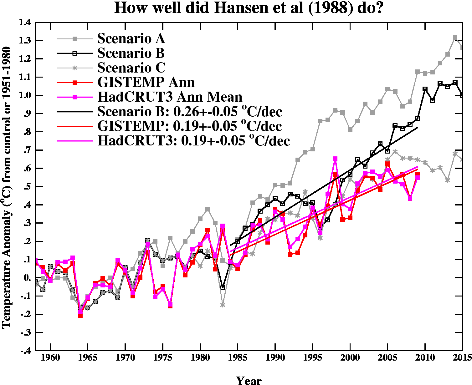
Figure 1: Global surface temperature computed for scenarios A, B, and C, compared with two analyses of observational data (Schmidt 2009)
What The Science Says:
Hansen's 1988 projections were too high mainly because the climate sensitivity in his climate model was high. But his results are evidence that the actual climate sensitivity is about 3°C for a doubling of atmospheric CO2.
Climate Myth: Hansen's 1988 prediction was wrong
'On June 23, 1988, NASA scientist James Hansen testified before the House of Representatives that there was a strong "cause and effect relationship" between observed temperatures and human emissions into the atmosphere. At that time, Hansen also produced a model of the future behavior of the globe’s temperature, which he had turned into a video movie that was heavily shopped in Congress. That model predicted that global temperature between 1988 and 1997 would rise by 0.45°C (Figure 1). Ground-based temperatures from the IPCC show a rise of 0.11°C, or more than four times less than Hansen predicted. The forecast made in 1988 was an astounding failure, and IPCC’s 1990 statement about the realistic nature of these projections was simply wrong.' (Pat Michaels)
In 1988, James Hansen projected future temperature trends using 3 different emissions scenarios identified as A, B, and C. Scenario A assumed continued exponential greenhouse gas growth. Scenario B assumed a reduced linear rate of growth, and Scenario C assumed a rapid decline in greenhouse gas emissions around the year 2000 (Hansen 1988). As shown in Figure 1, the actual increase in global surface temperatures has been less than any of Hansen's projected scenarios.
Figure 1: Global surface temperature computed for scenarios A, B, and C, compared with two analyses of observational data (Schmidt 2009)
As climate scientist John Christy noted, "this demonstrates that the old NASA [global climate model] was considerably more sensitive to GHGs than is the real atmosphere." Unfortunately, Dr. Christy decided not to investigate why the NASA climate model was too sensitive, or what that tells us. In fact there are two contributing factors.
A radiative forcing is basically an energy imbalance which causes changes at the Earth's surface and atmosphere, resulting in a global temperature change until a new equilibrium is reached. Hansen translated the projected changes in greenhouse gases and other factors in his three scenarios into radiative forcings, and in turn into surface air temperature changes. Scenario B projected the actual changes we've seen in these forcings most closely. As discussed by Gavin Schmidt and shown in the Advanced version of this rebuttal, the radiative forcing in Scenario B was too high by about 5-10%. Thus in order to assess the accuracy of Hansen's projections, we need to adjust the radiative forcing and surface temperature change accordingly.
Climate sensitivity describes how sensitive the global climate is to a change in the amount of energy reaching the Earth's surface and lower atmosphere (radiative forcings). Hansen's climate model had a global mean surface air equilibrium sensitivity of 4.2°C warming for a doubling of atmospheric CO2 [2xCO2]. This is on the high end of the likely range of climate sensitivity values, listed as 2-4.5°C for 2xCO2 by the IPCC, with the most likely value currently widely accepted as 3°C.
Since the Scenario B forcing was about 5-10% too high, its projected global surface air temperature trend was 0.26°C per decade, and the actual surface air temperature trend has been about 0.2°C per decade (NASA GISS), Hansen's climate model's sensitivity was about 25% too high. Thus the real-world climate sensitivity would be approximately 3.4°C to in order for Hansen's climate model to correctly project the ensuing global surface air warming trend. This climate sensitivity value is well within the IPCC range.
In other words, the reason Hansen's global temperature projections were too high was primarily because his climate model had a high climate sensitivity parameter. Had the sensitivity been approximately 3.4°C for a 2xCO2, and had Hansen decreased the radiative forcing in Scenario B slightly to better reflect reality, he would have correctly projected the ensuing global surface air temperature increase.
Hansen's study also produced a map of the projected spatial distribution of the surface air temperature change in Scenario B for the 1980s, 1990s, and 2010s. Although the decade of the 2010s has just begun, we can compare recent global temperature maps to Hansen's maps to evaluate their accuracy.
Although the actual amount of warming (Figure 3) has been less than projected in Scenario B (Figure 2), this is due to the fact that as discussed above, we're not yet in the decade of the 2010s (which will almost certainly be warmer than the 2000s), and Hansen's climate model projected a higher rate of warming due to a high climate sensitivity. However, as you can see, Hansen's model correctly projected amplified warming in the Arctic, as well as hot spots in northern and southern Africa, west Antarctica, more pronounced warming over the land masses of the northern hemisphere, etc. The spatial distribution of the warming is very close to his projections.
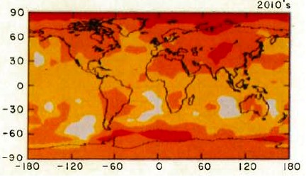

Figure 2: Scenario B decadal mean surface air temperature change map (Hansen 1988)
Figure 3: Global surface temperature anomaly in 2005-2009 as compared to 1951-1980 (NASA GISS)
The appropriate conclusion to draw from these results is not simply that the projections were wrong. The correct conclusion is that Hansen's study is another piece of evidence that climate sensitivity is in the IPCC stated range of 2-4.5°C for 2xCO2.
 |
The Skeptical Science website by Skeptical Science is licensed under a Creative Commons Attribution 3.0 Unported License. |