Climate Science Glossary

Term Lookup

Enter a term in the search box to find its definition.

Settings

Use the controls in the far right panel to increase or decrease the number of terms automatically displayed (or to completely turn that feature off).

Term Lookup

Settings


All IPCC definitions taken from Climate Change 2007: The Physical Science Basis. Working Group I Contribution to the Fourth Assessment Report of the Intergovernmental Panel on Climate Change, Annex I, Glossary, pp. 941-954. Cambridge University Press.

Home Arguments Software Resources Comments The Consensus Project Translations About Support

Twitter Facebook YouTube Mastodon MeWe

RSS Posts RSS Comments Email Subscribe


Climate's changed before
It's the sun
It's not bad
There is no consensus
It's cooling
Models are unreliable
Temp record is unreliable
Animals and plants can adapt
It hasn't warmed since 1998
Antarctica is gaining ice
View All Arguments...


Username
Password
New? Register here
Forgot your password?

Latest Posts

Archives

Hansen and Sato Estimate Climate Sensitivity from Earth's History

Posted on 24 May 2012 by dana1981

James Hansen and Makiko Sato from the NASA Goddard Institute for Space Studies (GISS) have made available a new draft paper, Climate Sensitivity from Earth's History (HS12).  The paper discusses reconstructions of global deep ocean temperature, sea level, surface temperature, and climate sensitivity going back thousands to millions of years.  HS12 is similar to a previous study, Hansen and Sato (2011) (HS11), but incorporates some updated data (e.g. revised radiative forcing estimates).  Here we will mainly focus on the surface temperature and climate sensitivity analysis in HS12 and its implications for the future of our climate.  We will see that HS12 provides an empirically-based climate sensitivity estimate which is consistent with estimates from today's climate models.  Figure 7 from HS12, our Figure 1 below, summarizes the authors' climate sensitivity conclusions.

HS12 Fig 7

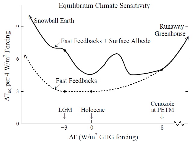
Figure 1:  Schematic diagram of the equilibrium fast-feedback climate sensitivity and Earth system sensitivity that includes surface albedo slow feedbacks.  Figure 7 from HS12.

In order to understand Figure 1, let's delve into some of the details of the paper.

HS12 Temperature Estimates

HS12 uses the oxygen isotope record in ocean sediments Zachos et al. (2008) to estimate past changes of sea level and ocean temperature, and thus obtain a largely empirical estimate of climate sensitivity.  HS11 (which is currently in press, and will actually be published in 2012) had used a previous version of that data set, publshed in 2001.  The Zachos 2008 data are shown in HS12 Figure 1, our Figure 2 below.

HS12 Fig 1

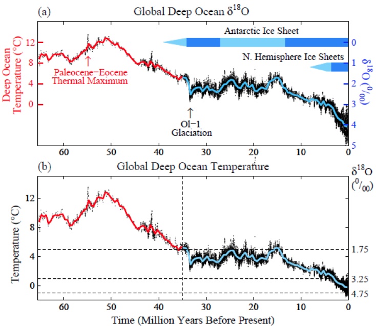
Figure 2: (a) Global deep ocean δ18O from Zachos et al. (2008) and (b) deep ocean temperature, with the latter based on the prescription in HS12. Black data points are 5-point running means of original temporal resolution; red and blue curves have 500 ky resolution.  Figure 1 from HS12.

Deep ocean temperature is approximated as linearly proportional to the fraction of the heavy oxygen istotope  (δ18O), though Hansen has concluded that the proportion depends on the size of the continental ice sheets.  As Earth became colder and continental ice sheets grew, further increase of δ18O was due in equal parts to deep ocean temperature change and ice mass change.

HS12 notes that as we are surface dwellers, the surface air temperature is of most interest to humans.  HS12 assume that deep ocean temperature change was similar to global mean surface temperature change for Cenozoic climates warmer than today, but this relationship does not hold true for colder climates.

"deep ocean temperature change does not provide a good indication of surface temperature change when the deep ocean approaches the freezing point, as quantified by Waelbroeck et al. (2002). The empirical data show that deep ocean cooling slows relative to global mean surface cooling as the area of ice and snow on the surface expands, consistent with the fact that the increase of δ18O between the Holocene and LGM was due more to ice sheet growth than to deep ocean cooling."

Last Glacial Maximum Temperature Change

The Last Glacial Maximum (LGM) approximately 20,000 years ago is a period often used to estimate climate sensitivity, because it represents a large climate shift in the relatively recent past, of which we have reasonably good measurements.

There have been a number of estimates of the average global surface temperature change during the LGM.  Most studies estimate the change close to 5°C, although there are some outliers, such as a paper we previously examined and which garnered a great deal of attention and misrepresentation from climate contrarians, Schmittner et al. (2011).  Schmittner et al. estimated the LGM cooling at only approximately 3°C, although as we discussed, this estimate was based heavily on sea surface temperature (SST) reconstructions from Multiproxy Approach for the Reconstruction of the Glacial Ocean (MARGO) project, which may underestimate the SST change.  This relatively low glacial-interglacial temperature change estimate contributed to the relatively low climate sensitivity estimate of Schmittner et al. (more on this below).

HS12 discusses another paper on the subject, Schneider von Deimling et al. (2006), which used an intermediate complexity climate model to estimate an LGM cooling of 5.8 ± 1.4°C, which is about twice as large as Schmittner et al., who fed their primarily MARGO-based temperatures into a climate model to estimate climate sensitivity.

Another paper we recently discussed, Shakun et al. (2012), estimated the global surface temperature change in the LGM cooling at 4.9°C.  HS12 reviews a number of other temperature estimates, including from the Vostok Antarctic ice core, and arrives at its LGM cooling estimate.

"Our estimate of LGM global cooling is thus 4.5±0.5°C, where 0.5°C is our estimated one standard deviation (σ) uncertainty. This range is meant to imply that there is about a 68% chance that the LGM global cooling was in the range 4-5°C, and about a 95% change that the cooling was in the range 3.5-5.5°C."

HS12 Implements an Empirical Approach

HS12 comments on the value of model-based results such as in the Schneider von Deimling and Schmittner studies.

"These model-based studies provide invaluable insight into the functioning of the climate system, because it is possible to vary processes and parameters independently, thus examining the role and importance of different climate mechanisms. However, the model studies also make clear that the results vary substantially from one model to another, and experience of the past few decades suggests that models are not likely to converge to a narrow range in the near future.

Therefore there is considerable merit in also pursuing a complementary approach that estimates climate sensitivity empirically from known climate change and climate forcings."

This empirically-based approach is the one Hansen and Sato pursue in this paper, while noting of course that their approach cannot be wholly independent of climate modeling, for example relying on radiative forcing computations from climate models, which is the most accurate way to estimate the magnitude of various forcings.  However, Hansen and Sato use climate models in a way that their climate sensitivity does not significantly influence their radiative forcing or the global temperature estimates that they use in this study.

"For example, the best global atmospheric models driven by specified sea surface temperatures can do a good job of simulating global temperature, winds and water vapor distributions. Thus such models can be used to help define the distribution of radiative constituents needed to calculate accurately the global climate forcing for alternative specifications of long-lived GHGs and surface albedo. Similarly, such global models can be used to help define global surface temperature for specified atmospheric composition and surface properties such as sea surface temperature."

In this manner, Hansen and Sato use climate models to help them estimate past radiative forcings and surface temperature changes using paleoclimate data without influencing their climate sensitivity estimates.  Thus their result in a predominantly empirical one.

Forcings vs. Feedbacks

One challenge in examining past climate data is in determining what should be treated as a forcing (driving a climate change) and what should be considered a feedback (amplifying or dampening a climate change).  Climate sensitivity is estimated by dividing the surface temperature change (which is influenced by both forcings and feedbacks) by the total radiative forcing (which does not include feedbacks).  Thus considering more temperature influences as forcings will increase the denominator, leading to smaller past climate sensitivity estimates, and vice-versa.

Aerosols are a challenge in this regard.  HS11 discussed that it would be best to treat natural aerosol emissions as a fast feedback rather than a forcing.

"There is nothing inherently wrong with defining aerosol changes to be a forcing, but it is practically impossible to accurately determine the aerosol forcing because it depends sensitively on the geographical and altitude distribution of aerosols, aerosol absorption, and aerosol cloud effects for each of several aerosol compositions. Moreover, aerosols adjust rapidly to a changing climate, so it is logical to include natural aerosol changes in the category of fast feedbacks.

The low estimates of climate sensitivity by Chylek and Lohmann (2008) and Schmittner et al. (2011), ~2°C for doubled CO2, are due in part to their inclusion of natural aerosol change as a climate forcing rather than as a fast feedback (as well as the small LGM-Holocene temperature change employed by Schmittner et al., 2011)."

Non-CO2 greenhouse gases (GHGs) could also be treated as either feedbacks or forcings.  In their estimate, Hansen and Sato only consider GHGs (including non-CO2 GHGs) and surface albedo (reflectivity) as forcings. 

"Our estimated LGM-Holocene forcings with 1σ uncertainties are 3±0.3 W/m2 for GHGs (range 2.4-3.6 W/m2 for 95% confidence) and 3±0.7 W/m2 for surface albedo (range 1.6-4.4 W/m2 for 95% confidence)."

Fast Feedback Climate Sensitivity Consistent with Climate Models

Hansen and Sato also differentiate between fast feedback and longer-term climate sensitivity, as illustrated in Figure 1 above.  Ice sheets can take centuries to millennia to melt or form, whereas sea ice changes occur much more rapidly (as we're currently seeing in the Arctic).  Therefore, albedo changes associated with sea ice are included in the fast feedback climate sensitivity, whereas albedo changes associated with ice sheets are only included in longer-term climate sensitivity estimates (which is termed "Earth System Sensitivity").

Thus given a total radiative forcing between the LGM and Holocene of approximately 6 W/m2, and a surface temperature change of approximately 4.5°C, HS12 arrives at a climate sensitivity best estimate of 3±0.5°C for a 4 W/m2 forcing (which is approximately equivalent to a doubling of atmospheric CO2).   While this value is consistent with today's model-based estimates, Hansen and Sato note,

"the empirical paleoclimate estimate of climate sensitivity is inherently more accurate than model-based estimates because of the difficulty of simulating cloud changes (NYTimes, 2012), aerosol changes, and aerosol effects on clouds."

The NYTimes reference in this quote is to the piece by Justin Gillis which we previously examined.  While climate contrarians like Richard Lindzen tend to treat the uncertainties associated with clouds and aerosols incorrectly, as we noted in that post, they are correct that these uncertainties preclude a precise estimate of climate sensitivity based solely on recent temperature changes and model simulations of those changes. 

However, as Hansen notes, empirical estimates of climate sensitivity based on paleoclimate data are consistent with the sensitivity in climate models of approximately 3°C for doubled atmospheric CO2.  In fact, as Figure 3 shows, the fit to the temperature data when multiplying the estimated radiative forcing by a climate sensitivity of 3°C for doubled CO2 is remarkably good.

HS12 Fig 6

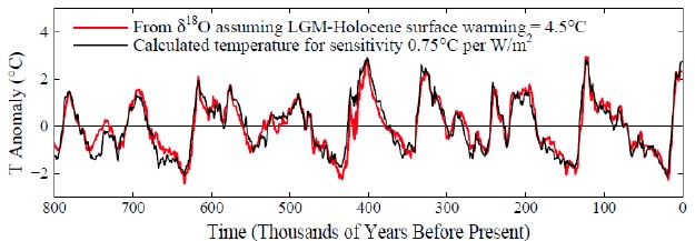
Figure 3: Black curve: calculated surface air temperature change for climate forcings in HS12 and climate sensitivity 0.75°C per W/m2. Red curve: estimated global surface air temperature change based on deep ocean temperatures and assumption that LGM-Holocene surface temperature change is 4.5°C. Zero point is the 800 ky mean.  Figure 6 from HS12.

Earth System Sensitivity

Hansen and Sato examine the longer-term Earth System Sensitivity by adding in slow feedbacks one-by-one, starting with surface albedo.  Hansen and Sato note the longer-term sensitivity is

"...more dependent on the initial climate state and the sign of the forcing. The fast-feedback climate sensitivity is a reasonably smooth curve, because the principal fast-feedback mechanisms (water vapor, clouds, aerosols, sea ice) do not have sharp threshold changes. Minor exceptions, such as the fact that Arctic sea ice may disappear with a relatively small increase of climate forcing above the Holocene level, might put a small wave in the fast-feedback curve."

This initial state dependency is illustrated by the more complex shape of the upper curve in Figure 1 above.  For example, during a cooling event to a glacial period like the LGM, the long-term Earth System Sensitivity is approximately 6°C for an equivalent forcing to a doubling (or in this case halving) of CO2.  This is primarily due to the increase in the Earth's reflectivity as large ice sheets form.

During a period like the Holocene while warming to a Pliocene-like climate, slow feedbacks (such as reduced ice and increased vegetation cover) increase the sensitivity to around 4.5°C for doubled CO2.  However, a climate warm enough to lose the entire Antarctic ice sheet would have a long-term sensitivity of close to 6°C.  Fortunately it would take a very long time to lose the entire Antarctic ice sheet.

Note also that the Earth System Sensitivity is deduced from various past climate change events like the Paleocene–Eocene Thermal Maximum (PETM), but the qualitative estimates of longer-term climate sensitivity are less precise than the HS12 fast feedback sensitivity estimates.  Hence the authors note that Figure 1 above is a schematic.

Summary

Hansen and Sato argue that the probable range of climate sensitivity values is not as large as currently believed (unlikely to fall outside the range of 2 to 4°C for doubled CO2) - both very high and very low values can effectively be ruled out using paleoclimate data.  This is also a position advocated by James Annan using a statistical approach, for example.  Climate contrarians often argue that model-based climate sensitivity estimates are unreliable and empirical estimates suggest that climate sensitivity is low.   On the contrary, HS12 shows that empirical estimates are consistent with climate models (as has also been previously shown by Knutti and Hegerl, for example [Figure 4]).

Various estimates of climate sensitivity

Figure 4: Distributions and ranges for climate sensitivity from different lines of evidence. The circle indicates the most likely value. The thin colored bars indicate very likely value (more than 90% probability). The thicker colored bars indicate likely values (more than 66% probability). Dashed lines indicate no robust constraint on an upper bound. The IPCC likely range (2 to 4.5°C) and most likely value (3°C) are indicated by the vertical grey bar and black line, respectively.  Adapted from Knutti and Hegerl (2008).

In short, all lines of evidence point to a climate sensitivity of close to 3°C for doubled CO2, which in turn points to a very dangerous amount of global warming if we continue on a business-as-usual path.

0 0

Printable Version  |  Link to this page

Comments

Comments 1 to 40:

  1. HS12 narrowing the error margins on their CS value to +/- 0.5 C is pretty significant compared to previous values more like +/- 1.5 C. If their methodology stands up to scrutiny this is quite useful. And it should make the cut for AR5.
    0 0
  2. The recent Hansen and Sato papers are easy to read, make very simple arguments, and are very compelling. The thing I can't judge as an outsider of course is whether his selection of source data realistically reflects the range of estimates in the field, and as a result if he is realistically including all the uncertainties. Someone who is more deeply read in the paleoclimate literature might be able to comment on that. I'd be interested to see a robust critique, but I don't remember any examples of anyone taking on Hansen in the primary literature. And I'm slightly bothered by how round the numbers always are. S_ff is always 3C, and the uncertainty is always a round number. That's a stupid criticism, because it's probably just a desire not to implicitly suggest a greater precision, but it bothers me slightly.
    0 0
  3. Very interesting paper that shows the dependency of historical climate forcing sensitivity on the accuracy of the historical temperature reconstruction used. As Hanson and Sato say themselves: "Global temperature change calculated by multiplying the sum of the two climate forcings in Fig. 5c by climate sensitivity ¾°C per W/m2 yields a remarkably good fit to the "observed" temperature (Fig. 6). The observed temperature is based on the assumption that 4.5°C is a reasonable approximation of the LGM-Holocene surface temperature change, and thus a scale factor of 2 is used to convert δ18O deep ocean temperature change (equation 6) to surface temperature change. However, we could obtain an equally good match between the temperature calculated from the forcings and the temperature from δ18O if we assumed the LGM-Holocene warming was 6°C and fast-feedback climate sensitivity was 1°C per W/m2, or if we assumed that the LGM-Holocene warming was 3°C and climate sensitivity was 0.5°C per W/m2. If LGM cooling is so uncertain as to be anywhere in the range 3-6°C, we can only conclude that the fast-feedback climate sensitivity is 3 ± 1°C for a 4 W/m2 CO2 forcing. Thus accurate knowledge of the global temperature change between glacial and interglacial states is needed for empirical evaluation of fast-feedback climate sensitivity." So their 3±0.5°C for a 4 W/m2 CO2 at 68% probability looks like it is directly based on their estimate of LGM global cooling being 4.5±0.5°C at 68% probability. Therefore I think the really interesting part of their paper is the Fig7 Equilibrium Climate Sensitivity chart more than the narrowed sensitivity itself.
    0 0
  4. Thanks Macoles, I hadn't picked up on the significance of that point. That goes a long way to addressing my question.
    0 0
  5. This is the first study I've seen which attempts to determine a complete spectrum of sensitivity values for all forcings relative to the current climate state. The finding that a 'runaway greenhouse' scenario would require greater than 8 W/m^2 forcing (i.e. two 'doublings' of CO2e, or 1120 ppm) is 'comforting' as that seems likely to be towards the upper end of our possible range of GHG forcing. That is, the point at which we would slip into a runaway greenhouse effect seems to be well beyond the point at which the damage caused by 'constrained' greenhouse warming would be sufficiently catastrophic to end further anthropomorphic GHG accumulations. I.E. it doesn't matter how stupid we are... we can't wipe ourselves out with fossil fuels alone. Yay? Presumably the prominent 'bump' in the equilibrium climate sensitivity at ~2-4 W/m^2 forcing is the albedo shift from the melting of Greenland and Antarctica. That's also very significant as it indicates that a 4 W/m^2 forcing sustained for thousands of years, which at this point is entirely possible, would result in the melting of the polar ice caps and the geological end of the Pleistocene epoch / current ice age. That would constitute a truly 'Anthropocene' geological epoch. One item of immediate concern is the convergence of the fast feedback and equilibrium sensitivity values at ~8 W/m^2 forcing. Does that suggest that the polar ice caps could melt within a hundred years at sustained 8 W/m^2 forcing? If so, we could be looking at a radically different world map by 2200.
    0 0
  6. "our present assessment of global LGM cooling must be partly subjective" (HS12) I don't see that much difference between Schmittner and HS12 except with regard to the quote above. Hansen likes the land paleo data more than ocean and as Schmittner shows his land based CS estimate is about inline with Hansen's.
    0 0
  7. HR @6 - Hansen's temperature estimates in this case are based on deep ocean δ18O.
    0 0
  8. HumanityRules @6, Hansen & Sato's estimate of 3 degrees C per 4 Watt/meter squared of forcing is equivalent to 2.8 C per doubling of CO2 (1 sigma uncertainty - 2.3-3.2 C). That would be closer to splitting the difference between Schmittner et al's land and ocean estimates.
    0 0
  9. Dana, I believe your first section is insufficiently clear. H&S 2012 refine their previous estimates of the fast feedback climate sensitivity using empirical data over the last 800,000 years. However, there representation of slow feedback climate sensitivity is characterized as a "schematic", and is not an empirical result. They highlight certain empirical events such as the PETM, and from features of those events, deduce qualitative features of the Slow Feedback Climate Sensitivity - but that does not make that figure an empirical conclusion. As an example, the entire justification peculiar peak in the center of the Fast Feedbacks plus Albedo curve (just to the right of holocene conditions is:
    "Also, in sketching the Earth system climate sensitivity we bear in mind the possibility of a hysteresis effect that makes demise of the Antarctic ice sheet difficult, thus stretching out toward larger forcing the ice sheet addition to the fast-feedback sensitivity."
    Hysteresis with respect to the Antarctic Ice sheet is probably a significant factor in Earth System Sensitivity, but it may modify the curve by first depressing it than elevating it, ie, by introducing a sine wave pattern rather than a simple peak. The reasoning does not even justify the shape of the curve, let alone the magnitude of the effects. I do not fault Hansen and Sato on this, as they are quite clear that their figure 7 (your figure 1) is a "schematic". I think that important qualification is eroded, however, when you describe the graph as their "climate sensitivity conclusions".
    0 0
  10. Dana says "HR @6 - Hansen's temperature estimates in this case are based on deep ocean δ18O." Are you sure? We are both talking about the LGM section of the paper? We're Hansen talks about "the less ambiguous terrestrial data" and where he criticizes Schmittners use of MARGO (oceanic) data? The deep ocean stuff seems to relate to the Cenozoic part of the paper.
    0 0
  11. Tom @9 - the first section is just an introduction, and Figure 1 is labeled as a schematic in the caption. However, I have added a note about the greater uncertainty regarding long-term sensitivity in the ESS section in the post.
    0 0
  12. (Section 5 of Hansen's paper)
    0 0
  13. HR @10 - yes, HS12 only uses ocean core data for their temperature reconstruction. In the section you quote they're only talking about other studies.
    0 0
  14. From section 5 "Our estimate of LGM global cooling is thus 4.5±0.5°C," "Our estimated LGM-Holocene forcings with 1σ uncertainties are 3±0.3 W/m2 for GHGs" I'd agree they are deriving these figures from a 'review' of other work but they seem to be presenting there own opinion as well. The second quote you use is from this section also. It actually seems like a strange add-on to the paper, I'm not sure of the purpose of it.
    0 0
  15. dana, thank you for clarifying about the qualitative nature of the ESS. With regard to your discussion with HR, I believe he has overstated his case, but is correct that H&S use terrestrial data in determining the climate sensitivity. H&S use the ocean core data to establish relative temperature over the last 800,000 years, and show that, with their estimated forcings and a fast feedback sensitivity of 3 degrees C per 4 W/m^2 of forcing, predicted and observed temperatures correlate near perfectly. However, as they note, an equally good correlation would be achieved if temperatures and sensitivity were each scaled by the same factor. Therefore, different assumptions about global temperatures at the LGM result in different, and consistent estimates of the fast feedback sensitivity. As they say:
    "Global temperature change calculated by multiplying the sum of the two climate forcings in Fig. 5c by climate sensitivity ¾°C per W/m^2 yields a remarkably good fit to the "observed" temperature (Fig. 6). The observed temperature is based on the assumption that 4.5°C is a reasonable approximation of the LGM-Holocene surface temperature change, and thus a scale factor of 2 is used to convert δ 18 O deep ocean temperature change (equation 6) to surface temperature change. However, we could obtain an equally good match between the temperature calculated from the forcings and the temperature from δ 18 O if we assumed the LGM-Holocene warming was 6°C and fast-feedback climate sensitivity was 1°C per W/m^2 , or if we assumed that the LGM-Holocene warming was 3°C and climate sensitivity was 0.5°C per W/m^2. If LGM cooling is so uncertain as to be anywhere in the range 3-6°C, we can only conclude that the fast-feedback climate sensitivity is 3 ± 1°C for a 4 W/m^2 CO2 forcing. Thus accurate knowledge of the global temperature change between glacial and interglacial states is needed for empirical evaluation of fast-feedback climate sensitivity."
    In order to constrain the temperatures at the LGM, Hansen and Sato discuss a variety of estimates, noting the inconsistency of sst based estimates such as CLIMAP and MARGO and terrestrial proxies. Finally, they state:
    "Given the inconsistencies among proxy data sets, our present assessment of global LGM cooling must be partly subjective. Our central estimate, 4.5°C, chosen with cognizance of discussions in the past three decades as new data sets were compared with CLIMAP, is in the middle of the range in the paleoclimate literature. Given that a global atmospheric model driven by CLIMAP sea surface temperatures yields LGM cooling of 3.6°C (Hansen et al., 1984), and indications that CLIMAP sea surface temperatures are incompatible with terrestrial data as well as with some marine data, we believe it is unlikely that global LGM cooling was much less than 4°C. On the high side, we argue that it is unlikely that global LGM cooling was much more than 5°C, because (1) LGM Antarctic cooling averaged over the Vostok (Vimeux et al., 2002) and Dome C (Jouzel et al., 2007) sites was 8-9°C, while both climate models and empirical data typically yield polar amplifications of quasi-equilibrium temperature change close to a factor of two, (2) despite disagreements about LGM ocean temperatures, there is general agreement that LGM cooling was limited in the tropics and subtropics."
    Thus they explicitly adopt an estimate greater than those based on CLIMAP and MARGO, and explicitly do so because of the inconsistencies with terrestrial data. However, they do not simply adopt an estimate based on terrestrial data, which would lead to a temperature estimate for the LGM closer to 6 degrees C below the pre-industrial average.
    0 0
  16. Fair point Tom, they certainly consider various LGM temperature reconstructions which use both terrestrial and ocean data.
    0 0
  17. @HumanityRules, #6 03:13 AM on 24 May, 2012: It is hard to to see how the Schmittner curves mix. (snip)
    0 0
    Moderator Response: TC: Of topic text snipped. I would greatly enjoy further exploration of the snipped text in a thread where it is on topic. Unfotunately it is off topic here, and consistency requires that I moderate based on compliance with the comments policy, not personal agreement or disagreement with points being made.
  18. Hi Newbie Physics guy, non climate guy interested in teaching this stuff here: Pointing out something that might possibly relate the 1981 Hansen, et al Science paper to this recent determination of sensitivity by fitting to past data? In 1981 paper, CO2 alone gives 1.2 degrees no feedbacks. (Model 1) By holding relative humidity constant ( water vapor feedback) sensitivity increased to 1.9 C. ( Hansen model 2)So 1.9 - 1.2 is 0.7 degrees which is 0.58 times the 1.2. Then if you just take these two effects alone why don't you get the real sensitivity = 1.2 (1 + .58 + .58^2 + etc) which by this being a geometric series gives 1.2 / (1-.58) = 2.9 degrees C? Which is about the same as the fitted climate sensitivity from Hanson and Sato?????? Or is this non runaway water vapor thing here already taken into account by the method of Hanson and Sato? Also does not this way of looking at it mean that it is a darned good thing that the "water vapor constant relative humidity assumption" gives 0.7 extra degrees , instead of twice that?, which would be more than the original 1.2 degrees? 1.2 / (1-..
    0 0
  19. O.K. I waded into one of the threads here on runaway greenhouse etc and found an incredible hornets nest of advanced electrical engineering analogues. Also found - I think - versions of my argument above which involves the simplest feedback model, maybe, with a positive feedback that is less than unity. So let me sharpen my question....does the real climate sensitivity include this effect of adding up increasingly smaller positive feedback terms in the water vapor feedback? Do real climate modelers include this effect?
    0 0
  20. Electrical engineers see feedback and try to construct climate in terms of something they know. With multiple non-linear feedbacks operating on different time-scales, it doesnt work well. What you ask would happen - but implicitly - as at each time-step in the model, the systems would respond to current temperature. Note also the AR4 models did not include carbon-cycle feedback (what would big for ice-age) as far as I know. This is because feedback is assumed to be too slow to have much effect in the next 100 years. I believe some AR5 models are full earth system model with a carbon cycle. (I am echoing comments heard from climate modellers sorry which isnt the most reliable source).
    0 0
  21. curiousd What do you mean by 'real climate sensitivity'? There are three different 'lengths' of climate sensitivity. A) Transient Climate Response (TCR) is the warming due to CO2 equiv at the point at which CO2 concentration has doubled, assuming a 1%/yr increase. Central estimate is around 2.0. B) Fast-Feedback/Equilibrium Climate Sensitivity (ECS), the most used definition, takes quite a while to realise (hundreds of years after doubling) and includes the diminishing positive feedback due to water vapor and sea ice albedo. Central estimate is around 3.0. C) Earth System Sensitivity includes the slow feedback resulting from large-scale glacial retreat and the long-term ocean responses. It could be as much as twice the ECS and takes thousands of years to realise.
    0 0
  22. 19, curiousd, The short answer to your question is "yes." The long answer is that climate sensitivity (in addition to Tristan's distinction between transient, fast feedback and Earth System) is a lot of different things, because it doesn't really exist as some fixed universal constant. As explained previously, every system configuration will respond differently. In casual conversation and for simple box models we use a single scalar to represent sensitivity relative to a doubling of CO2. But in a physics based climate model, for instance, you don't tell it the sensitivity, you tell it how atmospheric water vapor responds to a change in temperature, and how temperature responds to a change in water vapor... and a hundred other things. Then the model plays out and tells you what the climate sensitivity is in that scenario, as a (grossly oversimplified) scalar value. So to answer your question more directly, if you are talking about a climate model, the non-runaway-vapor-thing is included as a matter of physics, and if you're talking about a simple scalar value from paleoclimate or other observational study, the non-runaway-vapor-thing is included because you're looking at the "end result difference," and if it's a value computed in some other way it includes the non-=runaway-vapor-thing unless the person who put the number together was stupid.
    0 0
  23. O.K. think I kind of dig it, esp thanks scaddenp who points out about the time step in the computer models respond to each temperature so the kind of effect I am talking about is IMPLICITLY calculated. One follow up question...I get the feeling from the old 1981 Hansen paper that his water vapor feedback on the CO2 initial temperature increase is positive but less than unity which is a really good thing!! The temp of the earth if no greenhouse gases would be given by (S is solar constant) S/4 = emissivity x stef boltz const x T^4, so the surface area of the earth cancels out. But if the surface area of the earth were larger, and it contained proportionally more water, then once the greenhouse effect were taken into account I suspect you could get closer to a runaway condition, even if distance from sun is same as in real case. Yes? No? (Here I am trying to see the kinds of things that go into the modeling....probably one of them is how much water there is on earth?)
    0 0
  24. curiousd, No. It's really, really hard to get to a runaway. It has nothing to do with the surface of the earth, or how much water. Surface area means nothing, (everything is in units per square meter, it doesn't matter how many square meters in total). There's more than enough water on earth, too, the problem isn't that the system runs out of water. But there are negative feedbacks in place as well, the largest of which is the Planck effect... the hotter it gets, the more it radiates (power of 4), so it gets harder and harder to push that envelope. The "doubling" rule of CO2 applies to water vapor as well. Then there's the lapse rate feedback... as the earth warms, the lapse rate changes, and it becomes easier to radiate energy to space (i.e. more of the temperature change is higher up, where it can escape more easily to space). In the end, achieving a runaway is really, really hard. On how much water there is on earth... enough, but just for fun look at this.
    0 0
  25. Here's the image from that link, changed to also include the atmosphere rolled into a ball alongside the oceans. Note that all of the biomatter on earth is an almost invisible spec, the size of one pixel, in this image:
    0 0
  26. curiousd @23, relative humidity tends to be greater over ocean than over land, so increasing the surface area of the Earth's Oceans would indeed increase the relative strength of the Water Vapour feedback. It would also increase the strength of the negative feedback from the Lapse Rate feedback, which is the reduction of the Lapse Rate with increased humidity. The two effects do not cancel out, so that if the Earth was a 100% water world it would be warmer, all else being equal. However, it would not be sufficiently warm to initiate a runaway-greenhouse effect. The reasons why are discussed by Chris Colose here. The essence of the argument is that positive feedbacks reduce the outgoing radiation for a given surface temperature. If, but only if, the positive feedback reduces the OLR such that arbitrarily large increases of surface temperature are required to match the incoming solar radiation will you get a runaway feedback. For the Earth, with the water vapour/lapse rate feedback, effective insolation (insolation*(1-albedo) would need to be just over 320 W/m^2 rather than the current 240 W/m^2. The effective insolation needed to reach runaway greenhouse is called the Kombayashi-Ingersoll limit. Put another way, the Earth will only achieve a runaway greenhouse effect with current insolation if its albedo is reduced to 0.05 (give or take a bit for uncertainties).
    0 0
  27. Input wanted on Hansen's year 2000 article in Proc.Nat. Acad. Sci 97, pp. 9874 - 9880. Please!! Here he says "..rapid warming in recent decades has been driven mainly by non-CO2 greenhouse gases (GHGs), such as chlorofluorocarbons, CH4, and N2O, not by the products of fossil fuel burning, CO2 and aerosols."" Wow folks, doesn't this contradict the seminal 1981 paper? What happened here?????
    0 0
  28. curiousd @27, if you want a record of the changes in forcings from different GHG over the last three decades, go here. You will see that CH4 and NO2 forcing rose consistently through to about 1998, after which CH4 forcing leveled of while NO2 continued to rise. In contrast, CO2 forcing rose slowly during the 1990s, but sharply after 2000. Consequently, and contrary to expectations, CO2 was less important as a contributor to warming in the 1990s than it was in preceding decades, and in the 2000s. That in no way challenges Hansen 81. Climate scientists do not, by virtue of their expertise, claim any greater ability to predict things like the collapse of the Soviet Union (the cause of reduced CO2 emissions in the 1990s) or global financial crises. That is why they make projections conditional on certain plausible scenarios of growth in forcings rather than predictions. Of course, fake "skeptics" insist, implicitly, that AGW is falsified because Hansen did not predict that when Reagan said, "Tear down this wall", Gorbachov did so; or that the early 2000's would be dominated by El Ninos while the last few years have been dominated by La Ninas. Real skeptics are more sensible than that.
    0 0
  29. Questions on great Hanson and Sato paper: 1. They estimate Albedo from sea level since the sea level is determined by the major ice sheets. Clever!! Sea level is unaffected by floating ice packs, of course, such as ice now floating in the Arctic (but not for long, unfortunately). So does this mean that the contribution of the Arctic sea ice pack to the albedo is negligible compared to Greenland and Antarctica? 2. How does one determine sea levels going back 800,000 years?
    0 0
  30. Past sealevel is important for determine land/sea boundaries in albedo estimates. In a glacial period, the ice-sheets on Eurasia and North America are major contributors to albedo. Antarctica and Greenland were frozen then as now so dont contribute much to change in albedo. Ice extent is from geomorphology etc. Sea ice extent is inferred from plankton in sediment core. Some species only occur in open water, others under ice. This leads to chemical biomarkers too. I dont have the papers but putting "sea ice biomarker" into scholar.google.com will give quite a few papers. There are a number of techniques used to infer paleo sealevel. Try here for coral reef work. Have you had a look at Chpter 6 of the AR4 IPCC? This links to many papers on this topic.
    0 0
  31. By the way, the albedo estimates and modelling used go back to Hansen et al 2007, which for input relies heavily on the accumulated data from multiple sources in CLIMAP 1981.
    0 0
  32. To someone who needs to explain/impress both smart but non technical students, and to physics phds who are nearly ignorant of climate change, that figure 3 above could be a "game changer". The agreement between experiment and theory is rather like one sees in many areas of condensed matter physics. For instance it is like one obtains in fitting extended x-ray fine structure (EXAFS)data to a structural model. But one needs to know the number of adjustable parameters. When I first read the article, I thought that since they were able to figure out the albedos, CO2 concentrations, and temperatures that that figure represents only one adjustable parameter, the short term (transient) CO2 climate sensitivity. Now I am not so sure because of the mention of the N2O and CH4. In EXAFS theory a big deal is made about the number of independent data points and the number of adjustable parameters. If it is only one (or two ) (or three) parameters that are being fitted here the result is spectacular. (Nobel Prize Hanson?) Any help on what you think the number of adjustable parameters is? BTW...he gets rid of the "clouds" uncertainty by this empiricle method, right? Another "Lindzen ism" dealt with?
    0 0
  33. curiousd - my understanding of the calculated temperature in Fig 3, is that depends on only 3 inputs - CH4, CO2 and sealevel. However, they are are not directly "fitted" to a curve. N2O is also important but not preserved, but because it strongly correlated with CO2 and CH4, its contribution is added in as a 1.12 multiplier on the forcing strength of CO2 + CH4. This no. being consistent with radiative codes. Albedo is sum of a great many changes - ice shelves, ice sheets, changing land/ocean ratios, changing vegetation, but the earlier work (2007 from CLIMAP 1981) showed that it could estimated by sealevel alone as a "good enough" approximation. Clouds are problematic but clouds have both positive and negative effects and net forcing for current time is thought to be close to zero. There is no proxy for clouds but this data is at least consistent with assumption that net contribution has been very small compared to GHG and albedo. Note the cause of the ice-age cycle is solar variation but solar forcing isnt included. The global solar forcing is very small but the regional distribution means that it is expressed an albedo forcing. Note also, that the climate sensitivity that produces the good fit is dependent on 4.5C temp difference between LGM and Holocene. Use a different temp diff and you get a different sensitivity as discussed in detail in the paper.
    0 0
  34. Just one other note - a global average temperature isnt really that complex a thing. For any planet rotating fast enough to equilibrate temperatures, then surface temp is function of incoming solar radiation, planetary albedo, geothermal heatflux (insignificant on earth) and atmospheric composition (GHG). eg a calculator or here for some of the equations. The tricky bit is predicting how atmosphere composition and albedo will change if alter something.
    0 0
  35. Maybe I now know enough to make a slight correction to something someone told me(not sure who the someone was) here in one of many helpful answers to my questions. The recent pre print Hansen and Sato made available here states they determine a "fast feedback" response which includes CO2, water vapor feedback, sea ice, clouds, aerosols. The warming up of the entire ocean, (like the melting of Antarctica and Greenland)is longer term, on order of "100s of years" Someone - I think incorrectly - confused fast feedback response, which is a portion of the equilibrium response, with the "transient response". "Transient response" means you run a simulation to include continual addition of CO2, which, unfortunately, is what "really happens". Also, the warming up of the ocean is not included in either the fast feedback response or the transient response because it can take 1000 years for the ocean temperature to equilibriate with the surface?? Do I now have this right?
    0 0
  36. curiousd @35, transient climate response (TCR), the Charney Sensitivity, aka, the Equilibrium Climate Sensitivity (ECS), and the Earth System Sensitivity (ESS) all have clear definitions in computer models. The Earth System Sensitivity is the change in temperature with a doubling of CO2 with constant forcing after the system has reached equilibrium, allowing all feedbacks fast and slow to operate. The Equilibrium Climate Response is the change in temperature with doubled CO2 and constant forcing after the system has reached equilibrium with only fast feedbacks allowed to operate. The transient climate response is the average temperature in the twenty year interval centered on the year that CO2 reaches double the initial value when it is increased by 1% per annum throughout the model run. Outside of models, we cannot control things so easily. CO2 increases at greater than 1% per annum, and not be the same percentage each year. Fast feedbacks and slow feedbacks both occur. However, the TCR as scaled for the appropriate forcing still approximates to the current expected temperature during a period of increasing CO2. The scaled ECS still approximates to the temperature we can expect a hundred or so years after CO2 emissions begin to be held steady. And the scaled ESS approximates to the temperature the Earth will be at if CO2 concentrations are held near constant over thousands of years. In each case, however, they are only approximations. In any event, the time it takes for the deep ocean to warm is not a feedback. It is only a constraint on the response time.
    0 0
  37. Tom Curtis, I Love it! Thank you! You need to look for grains of humor in this deadly serious business, and so now I get to impress my "ordinary physics" prof colleagues with the delightful wonkiness of the ESS versus the EGS. So cool. (so to speak) So.....I guess by Hanson - Sato latest, the ECS is 3.0 degrees C plus or minus 0.5 degrees by their fit, at least. So is there a latest and greatest ESS? Or alternatively a cluster of results you could recommend for the ESS?
    0 0
  38. curiousd @37, Park and Royer (2011) is a good place to start. They find an ESS of 3 to 4 degrees C is a robust feature of the geological record during periods with no ice sheets at the the Earth's poles; and 6 to 8 C in periods with ice sheets at the poles. Hansen and Sato have also recently estimated ESS, but somebody else will have to provide the link.
    0 0
  39. On p.14 HS12 says: "[T]he mean sensitivity over the entire range from the Holocene to a climate just warm enough to lose the Antarctic ice sheet is almost 6°C for doubled CO2, but most of the surface albedo feedback in that range is caused by loss of the Antarctic ice sheet [...] [T]he sensitivity is smaller as climate warms from the Holocene toward a Pliocene-like climate. Thus the estimate of Lunt et al. (2010), that slow feedbacks (reduced ice and increased vegetation cover) increase the sensitivity by a factor of 1.3-1.5 is not inconsistent with the Hansen et al. (2008) estimated sensitivity." On p.15 they say: "If non-CO2 trace gases are counted as a fast feedback, the fast-feedback sensitivity becomes 4°C for doubled CO2, and the Earth system sensitivity becomes 8°C for doubled CO2 with the surface albedo feedback included [...] These sensitivities apply for today's initial climate state and negative climate forcings; they are reduced for positive forcings [...] The ultimate Earth system sensitivity includes all fast and slow feedbacks, i.e., surface feedbacks and all GHG feedbacks including CO2. Apparently Sff+sf is remarkably large in the Pleistocene for a negative forcing. No doubt that accounts for the substantial cooling of Earth in the past few million years in response to only small changes of CO2., as well as the increasingly violent glacial-to-interglacial oscillations of the late Pleistocene (Fig. 4). The Earth system sensitivity relevant to humanity now is the sensitivity of the present climate state to a positive (warming) forcing. That sensitivity is not as great as for a negative forcing, but it is much larger than the 3°C fast-feedback climate sensitivity." So do I understand correctly (from these quotes and their figure 7) that H&S think ESS for doubled CO2 over the past million years was more than 8 deg C and more than 6 deg for the current climate until all the ice has melted, after which it is reduced to somewhere between 4.5 and around 5 deg and rising again for even warmer climates? It seems I'm confusing sensitivities with and without CO2- and non-CO2 GHG-feedbacks. And H&S don't seem to give an estimate of the magnitude of the possible CO2-feedback. Does anyone have a clearer picture on this? How much more warming can we expect in the longer term when the CO2-feedback starts working? And how long would that term be: centuries or more like millennia?
    0 0
  40. A new paper by Friedrich et al. 2016 http://advances.sciencemag.org/content/2/11/e1501923   agrees with HS12 that averaged over all the paleo data, CS =3.2 C. However, the point of their paper is that CS is very nonlinear, and is small at cold temps and high at warmer temps. In fact, they find CS=4.88C at the interglacial highs. The dots of paleo data do show a convincing strongly arcing upward curvature in deltaT vs forcing. If this is true, this is a real game-changer in a bad way. Does anyone know of significant criticisms of the Friedrich work? A casual search doesn't find any.

    0 0

You need to be logged in to post a comment. Login via the left margin or if you're new, register here.


The Consensus Project Website

THE ESCALATOR

(free to republish)


© Copyright 2024 John Cook
Home | Translations | About Us | Privacy | Contact Us