Climate Science Glossary

Term Lookup

Enter a term in the search box to find its definition.

Settings

Use the controls in the far right panel to increase or decrease the number of terms automatically displayed (or to completely turn that feature off).

Term Lookup

Settings


All IPCC definitions taken from Climate Change 2007: The Physical Science Basis. Working Group I Contribution to the Fourth Assessment Report of the Intergovernmental Panel on Climate Change, Annex I, Glossary, pp. 941-954. Cambridge University Press.

Home Arguments Software Resources Comments The Consensus Project Translations About Support

Twitter Facebook YouTube Mastodon MeWe

RSS Posts RSS Comments Email Subscribe


Climate's changed before
It's the sun
It's not bad
There is no consensus
It's cooling
Models are unreliable
Temp record is unreliable
Animals and plants can adapt
It hasn't warmed since 1998
Antarctica is gaining ice
View All Arguments...


Username
Password
New? Register here
Forgot your password?

Latest Posts

Archives

A detailed look at Hansen's 1988 projections

Posted on 20 September 2010 by dana1981

Hansen et al. (1988) used a global climate model to simulate the impact of variations in atmospheric greenhouse gases and aerosols on the global climate.  Unable to predict future human greenhouse gas emissions or model every single possibility, Hansen chose 3 scenarios to model.  Scenario A assumed continued exponential greenhouse gas growth.  Scenario B assumed a reduced linear rate of growth, and Scenario C assumed a rapid decline in greenhouse gas emissions around the year 2000.

Misrepresentations of Hansen's Projections

The 'Hansen was wrong' myth originated from testimony by scientist Pat Michaels before US House of Representatives in which he claimed "Ground-based temperatures from the IPCC show a rise of 0.11°C, or more than four times less than Hansen predicted....The forecast made in 1988 was an astounding failure." 

This is an astonishingly false statement to make, particularly before the US Congress.  It was also reproduced in Michael Crichton's science fiction novel State of Fear, which featured a scientist claiming that Hansen's 1988 projections were "overestimated by 300 percent." 

Compare the figure Michaels produced to make this claim (Figure 1) to the corresponding figure taken directly out of Hansen's 1988 study (Figure 2).


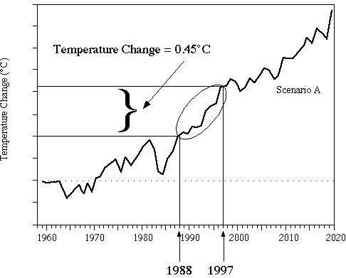
Figure 1: Pat Michaels' presentation of Hansen's projections before US Congress


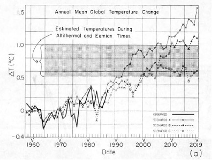
Figure 2: Projected global surface air temperature changes in Scenarios A, B, and C (Hansen 1988)

Notice that Michaels erased Hansen's Scenarios B and C despite the fact that as discussed above, Scenario A assumed continued exponential greenhouse gas growth, which did not occur.  In other words, to support the claim that Hansen's projections were "an astounding failure," Michaels only showed the projection which was based on the emissions scenario which was furthest from reality. 

Gavin Schmidt provides a comparison between all three scenarios and actual global surface temperature changes in Figure 3.


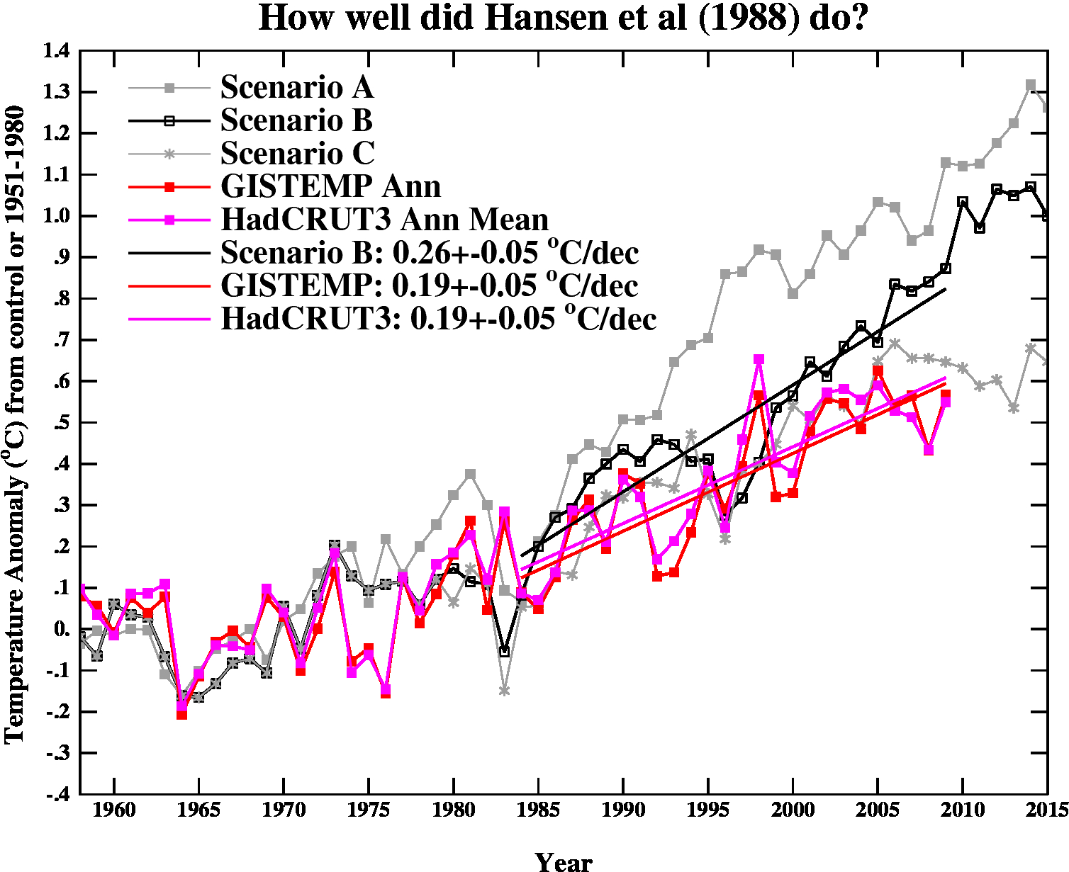
Figure 3: Hansen's projected vs. observed global temperature changes (Schmidt 2009)

As you can see, Hansen's projections showed slightly more warming than reality, but clearly they were neither off by a factor of 4, nor were they "an astounding failure" by any reasonably honest assessment.  Yet a common reaction to Hansen's 1988 projections is "he overestimated the rate of warming, therefore Hansen was wrong."   In fact, when skeptical climate scientist John Christy blogged about Hansen's 1988 study, his entire conclusion was "The result suggests the old NASA GCM was considerably more sensitive to GHGs than is the real atmosphere."  Christy didn't even bother to examine why the global climate model was too sensitive or what that tells us.  If the model was too sensitive, then what was its climate sensitivity?

This is obviously an oversimplified conclusion, and it's important to examine why Hansen's projections didn't match up with the actual surface temperature change.  That's what we'll do here.

Hansen's Assumptions

Greenhouse Gas Changes and Radiative Forcing

Hansen's Scenario B has been the closest to the actual greenhouse gas emissions changes.  Scenario B assumes that the rate of increasing atmospheric CO2 and methane increase by 1.5% per year in the 1980s, 1% per year in the 1990s, 0.5% per year in the 2000s, and flattens out (at a 1.9 ppmv per year increase for CO2) in the 2010s.  The rate of increase of CCl3F and CCl2F2 increase by 3% in the '80s, 2% in the '90s, 1% in the '00s, and flatten out in the 2010s. 

Gavin Schmidt helpfully provides the annual atmospheric concentration of these and other compounds in Hansen's Scenarios.  The projected concentrations in 1984 and 2010 in Scenario B (in parts per million or billion by volume [ppmv and ppbv]) are shown in Table 1.

Table 1: Scenario B greenhouse gas (GHG) concentration in 1984, as projected by Hansen's Scenario B in 2010, and actual concentration in 2010


GHG 

1984 

Scen. B 2010 

 Actual 2010

CO2  344 ppmv  389 ppmv  392 ppmv
N2O  304 ppbv  329 ppbv  323 ppbv
CH4  1750 ppbv  2220 ppbv  1788 ppbv
CCl3F  0.22 ppbv  0.54 ppbv  0.24 ppbv
CCl2F2  .038 ppbv  0.94 ppbv  0.54 ppbv


We can then calculate the radiative forcings for these greenhouse gas concentration changes, based on the formulas from Myhre et al. (1998).

dF(CO2) = 5.35*ln(389.1/343.8) = 0.662 W/m2

dF(N2O) =  0.12*(N - N0) - (f(M0,N) - f(M0,N0))

= 0.12*(329 - 304) - 0.47*(ln[1+2.01x10⁻⁵ (1750*329)0.75+5.31x10⁻¹⁵ 1750(1750*329)1.52]-ln[1+2.01x10⁻⁵ (1750*304)0.75+5.31x10⁻¹⁵ 1750(1750*304)1.52]) = 0.022 W/m2

dF(CH4) =0.036*(M - M0) - (f(M,N0) - f(M0,N0))

= 0.036*(2220 - 1750) - 0.47*(ln[1+2.01x10⁻⁵ (2220*304)0.75+5.31x10⁻¹⁵ 2220(2220*304)1.52]-ln[1+2.01x10⁻⁵ (1750*304)0.75+5.31x10⁻¹⁵ 1750(1750*304)1.52]) = 0.16 W/m2

dF(CCl3F) = 0.25*(0.541-0.221) = 0.080 W/m2

dF(CCl2F2) = 0.32*(0.937-0.378) =  0.18 W/m2

Total Scenario B greenhouse gas radiative forcing from 1984 to 2010 = 1.1 W/m2

The actual greenhouse gas forcing from 1984 to 2010 was approximately 1.06 W/m2 (NASA GISS).  Thus the greenhouse gas radiative forcing in Scenario B was too high by about 5%.

Climate Sensitivity

Climate sensitivity describes how sensitive the global climate is to a change in the amount of energy reaching the Earth's surface and lower atmosphere (a.k.a. a radiative forcing).  Hansen's climate model had a global mean surface air equilibrium sensitivity of 4.2°C warming for a doubling of atmospheric CO2 [2xCO2].  The relationship between a change in global surface temperature (dT), climate sensitivity (λ), and radiative forcing (dF), is

dT = λ*dF

Knowing that the actual radiative forcing was slightly lower than Hansen's Scenario B, and knowing the subsequent global surface temperature change, we can estimate what the actual climate sensitivity value would have to be for Hansen's climate model to accurately project the average temperature change.

Actual Climate Sensitivity

One tricky aspect of Hansen's study is that he references "global surface air temperature."  The question is, which is a better estimate for this; the met station index (which does not cover a lot of the oceans), or the land-ocean index (which uses satellite ocean temperature changes in addition to the met stations)?  According to NASA GISS, the former shows a 0.19°C per decade global warming trend, while the latter shows a 0.21°C per decade warming trend.  Hansen et al. (2006) – which evaluates Hansen 1988 – uses both and suggests the true answer lies in between.  So we'll assume that the global surface air temperature trend since 1984 has been one of 0.20°C per decade warming.

Given that the Scenario B radiative forcing was too high by about 5% and its projected surface air warming rate was 0.26°C per decade, we can then make a rough estimate regarding what its climate sensitivity for 2xCO2 should have been:

λ = dT/dF = (4.2°C * [0.20/0.26])/0.95 = 3.4°C warming for 2xCO2

In other words, the reason Hansen's global temperature projections were too high was primarily because his climate model had a climate sensitivity that was too high.  Had the sensitivity been 3.4°C for a 2xCO2, and had Hansen decreased the radiative forcing in Scenario B slightly, he would have correctly projected the ensuing global surface air temperature increase.

The argument "Hansen's projections were too high" is thus not an argument against anthropogenic global warming or the accuracy of climate models, but rather an argument against climate sensitivity being as high as 4.2°C for 2xCO2, but it's also an argument for climate sensitivity being around 3.4°C for 2xCO2.  This is within the range of climate sensitivity values in the IPCC report, and is even a bit above the widely accepted value of 3°C for 2xCO2.

Spatial Distribution of Warming

Hansen's study also produced a map of the projected spatial distribution of the surface air temperature change in Scenario B for the 1980s, 1990s, and 2010s.  Although the decade of the 2010s has just begun, we can compare recent global temperature maps to Hansen's maps to evaluate their accuracy.

Although the actual amount of warming (Figure 5) has been less than projected in Scenario B (Figure 4), this is due to the fact that as discussed above, we're not yet in the decade of the 2010s (which will almost certainly be warmer than the 2000s), and Hansen's climate model projected a higher rate of warming due to a high climate sensitivity.  However, as you can see, Hansen's model correctly projected amplified warming in the Arctic, as well as hot spots in northern and southern Africa, west Antarctica, more pronounced warming over the land masses of the northern hemisphere, etc.  The spatial distribution of the warming is very close to his projections.


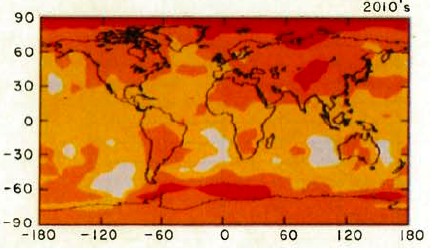
Figure 4: Scenario B decadal mean surface air temperature change map (Hansen 1988)


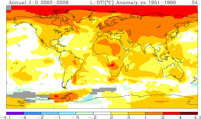
Figure 5: Global surface temperature anomaly in 2005-2009 as compared to 1951-1980 (NASA GISS)

Hansen's Accuracy

Had Hansen used a climate model with a climate sensitivity of approximately 3.4°C for 2xCO2 (at least in the short-term, it's likely larger in the long-term due to slow-acting feedbacks),  he would have projected the ensuing rate of global surface temperature change accurately.  Not only that, but he projected the spatial distribution of the warming with a high level of accuracy.  The take-home message should not be "Hansen was wrong therefore climate models and the anthropogenic global warming theory are wrong;" the correct conclusion is that Hansen's study is another piece of evidence that climate sensitivity is in the  IPCC stated range of 2-4.5°C for 2xCO2.

This post is the Advanced version (written by dana1981) of the skeptic argument "Hansen's 1988 prediction was wrong". After reading this, I realised Dana's rebuttal was a lot better than my original rebuttal so I asked him to rewrite the Intermediate Version. And just for the sake of thoroughness, Dana went ahead and wrote a Basic Version also. Enjoy!


0 0

Printable Version  |  Link to this page

Comments

1  2  3  Next

Comments 1 to 50 out of 135:

  1. Misprint on the first line. Says 1998; should be 1988.
    0 0
    Response: Fixed, thanks
  2. It is hard to look at Hansen's 1988 work without seeing he got it right! A few quibbles, but the major mechanisms are all included, and he is off by a few tenths of a degree over 22 years! And the fix is very clear - he used 4.2 instead of 3 or 3.4 for climate sensitivity. The takehome message is climate scientists have this dialed in. With 22 years more research, current models are that much better. "Hansen got it wrong" is a lie - pure and simple.
    0 0
  3. Heres some interesting analysis... http://residualanalysis.blogspot.com/2010/02/twin-ghgs-paradox.html The Twin GHGs Paradox The means by which a greenhouse gas (GHG) forces climate change is sometimes called radiative forcing.
    0 0
    Moderator Response: Please provide more context when you post a link.
  4. I wonder if you would consider typesetting the math with LaTeX? Would make it lots more readable. You could e.g. use http://www.codecogs.com/latex/eqneditor.php. Or if you already know LaTeX, just use TTH: http://hutchinson.belmont.ma.us/tth/
    0 0
  5. The other thing that I think should be pointed out is that Hansen scenario B was also taking into consideration a large volcanic eruption in 1995 while Pinatubo - which can be clearly seen in the actual data - was in 1991 - once you also correct for that the scenario B already looks identical to real measured values!
    0 0
  6. @paulm: That website proves nothing. Radiative forcing F is a multivariate nonlinear function. But for small variations, we can Taylor-expand and to first order it is the sum of the first derivatives. The particular objection raised is that for example d^2F/d(CO2)/d(N2O) is not zero. I agree it's not. But its contribution to dF is much smaller than the linear part. As it's unknown, it contributes to the uncertainty (error-bar) in the calculation.
    0 0
  7. One thing that folks should keep in mind is that your typical el-cheapo Best-Buy/Walmart/whatever laptop has more computing horsepower than what Hansen had available to him to conduct his climate-modeling simulations back in 1988. This should put things in perspective here, and also give folks a fuller appreciation of Hansen's genius.
    0 0
  8. Something here does not make sense. Nowhere do you mention what the actual emissions WERE over the intervening period. You cannot simply compare one of Hansen's scenarios with what actually happened in terms of outcomes, if you do not take into account the inputs. If the temperature curve nicely follows Hansen's scenario B, but the emissions increased exponentially (i.e., according to scenario A), Hansen's model was overestimating by a much larger margin.
    0 0
  9. Sense Seeker, you missed something. Two quotes from the post: "Scenario A assumed continued exponential greenhouse gas growth, which did not occur." "Hansen's Scenario B has been the closest to the actual greenhouse gas emissions changes."
    0 0
  10. Ricardo, you are mostly right but not completely. (Unless I missed something more, which is of course now a non-negligible option.) Shouldn't Table 1 give the realised Greenhouse Gas (GHG) Concentration in 1984 and 2010, rather than the one from Scenario B? The calculations seem to be based on scenario B, not the realised emissions. The real ones may be most like scenario B compared to A or C, but are unlikely to be identical. If you only want to test the model, you need to use the observed emissions as input.
    0 0
  11. Once the data for 2010 are used, his accuracy will have been prophetic.
    0 0
  12. And if you want to test Hansen's scenario B as a prediction, rather than the underlying model, you needn't bother with any calculation. You can just read if from the graph.
    0 0
  13. There is one more thing I don't understand. The calculations did not use Hansen's model, but a set of equations from a different source (Myhre et al 1998). Comparison with the forcings as established (beyond doubt, is seems) with an unexplained NASA method, and then conclude that Hansen's model was almost accurate... I am sorry, I can see Hansen got it about right, but this posting adds little to my understanding.
    0 0
  14. I clicked the link to NASA-GISS for the +1.1W/sq.m 2010 relative to 1984 forcing here: http://data.giss.nasa.gov/modelforce/RadF.txt and found data only to 2003 and nothing like +1.1. Please explain the calculation? My eyesight must be playing tricks for I see the actual temperatures running close or below Scenario C not Scenario B. Is that what you meant? And what of the climate responses - where is the estimate of WV and Ice albedo feedback and radiative cooling feedback? Seems like a contrived Hansen apologia with only half the story to me.
    0 0
  15. Sense Seeker, #10 in this post there's a comparison of Hansen's calculation in 1988 not a thorough comparison of model results. How could he know the actual emissions in the future? Someone else could do now some new calculations with actual emissions and best available model now, but this is a different story. A good idea for a new post ;) #13 the model is not on radiative forcing alone, it's much more than this; it is called a General Circulation Model (GCM). Radiative forcings come from radiative tranfer codes that are pluged into the GCMs. I think you should dig a little bit more on GCMs; NASA GISS provide a lot of informations (and the code itself) that I'm sure you'll find intersting.
    0 0
  16. Ken Lambert, it's way too easy to talk about apologia without even bothering to look at the details on how things work. This attitude just highlight the unwillingness to learn the science but still dismissing it. The feedbacks are, indeed, feedback, not forcings. Why should they be listed in the same table as the forcings? The albedo, water vapour feedbacks and others are the results of the full calculations and are not parametrized.
    0 0
  17. Riccardo #16 Unfortunately the measures 'air surface temperature' and GISS and HADCRUT3 temperature anomalies are the result of ALL the forcings - both radiative and feedbacks. Claiming that Hansen was out by only 5% on half the story when the feedbacks (particularly WV and CO2 interaction) are the least understood is the missing part of this article. So we are closest Scenario C with the temperature record??
    0 0
  18. First I want to say that to be able to come up with those projections in 1988 is remarkable. I think I was still using an Atari 800 at the time. Now this may be a stupid question but as discussed in a previous post, is the idea that we should be naturally cooling incorporated into the model. Of course I assume it is but just one of those nagging questions.
    0 0
  19. Ken Lambert, still confusing forcings and feebacks, do you? Anyway, Hansen calculation also are "the result of ALL the forcings - both radiative and feedbacks." (sic). And within 5%.
    0 0
  20. Scrooge, natural cooling is ignored in GCM. It happens on a time frame of millennia which usually is not considered.
    0 0
  21. Wonder if Michaels is going to retract the misleading and erroneous testimony that he gave before US House of Representatives? I mean in the spirit of accountability,transparency and rigor that he demands of the IPCC? Excellent job Dana. Am I correct in understanding that emission scenarios B and C were the same up until 2000?
    0 0
  22. A close look at Figure 3 shows that temperatures are actually running below Scenario C - the zero-increase in CO2 from 2000. This decline has not happened. Therefore, the only conclusion that can be made from present day temperature readings is that Hansen (1988 & 2006) got it wrong.
    0 0
  23. angusman #22, scenarios B and C and the actual temperature record are all very similar to each other through 2005. Since 2005 actual temperatures have been roughly in line with scenario C (below in some years, above in others). However, that is FAR too short a time frame on which to judge the validity of the model. If actual results continued tracking along scenario C for 15+ years then the model would be off significantly. If the warming being seen this year continued then we'd be back 'on track' closer to scenario B. That said, Hansen's 'short term' climate sensitivity factor in 1988 was definitely too high and thus his results should be expected to go further off as time goes by. Hansen 2006 essentially explained HOW the 1988 analysis got it wrong... so to say that 2006 is itself wrong... would seem to be arguing that Hansen 1988 was correct. :]
    0 0
  24. Sense Seeker - I didn't provide the actual atmospheric concentrations of the various GHGs, but I did provide the actual radiative forcing associated with them, which is what matters for these calculations. Also Hansen '88 provided his formulas for dT but not dF, so I used Myhre for the dFs, which are reasonably close to Hansen's values. Ken Lambert - as the GISS forcing link only provided data up to 2003, I extrapolated to 2010 to get a value of approximately 1.06 W/m2. Several commenters have stated that the actual temperatures have run close to Scenario C, which completely misses the point, and I would suggest re-reading the rebuttal. Actual emissions have not been very similar to Scenario C, so comparing to Scenario C rather than B doesn't make sense. Albatross - yes, Scenarios B and C were very similar (perhaps identical, I'd have to go back and look) up until 2000.
    0 0
  25. A night's sleep does help. I can see what you were trying to do. You are comparing the inputs of Hansen's scenario B (translated into forcings) and the actual changes in the input variables (as 'observed' forcings), and then compare Hansen's output (= projected temperatures) with the real output (= realised temperatures). From that you conclude that Hansen's model was 24% too sensitive. It is a pity that the detour via forcings is there, but I guess that is the best way to summarise all different emissions? (I cannot judge that.) You could consider explaining why the translation into forcings is necessary and justified; it was not obvious to me when I first read it. To guide the reader, you could also consider indicating somewhere in the beginning of your explanation what you are going to do, in broad terms. (Determine difference in input values (GHGs) and compare to differences in output (temp) between Hansen's model and reality.) PS: typo "global surface temperature (dF)" should be (dT)?
    0 0
  26. Youve lost me with this analysis... in the top graph, the closest is scenario C to observations... A and B appear to clearly over estimate climate sensitivity... Now B is the closest to observed emissions clearly, But C is the closest to observations, how can this mean anything other than an overstated climate sensitivity? Now it dosnt matter one iota what anyone's opinion is on what the temps "will be" in a decade, all that matters for testing the model is a straight comparison between projected and observations. It may be due
    0 0
  27. @Joe Blog: "how can this mean anything other than an overstated climate sensitivity" Isn't that the conclusion of the article, i.e. that Hansen overestimated climate sensitiviy (4.2C instead of 3.4C)?
    0 0
  28. archiesteel Yes, so Hansen was wrong, in his climate sensitivity. It certainly doesn't prove Hansens projections were accurate, or disprove criticisms of his projections, as the article claims to do.
    0 0
  29. Joe... You have to bear in mind this is coming from a study done in 1988 and it's an incredibly complex model. Given that Hansen managed to closely predict warming for the following 22 years is astounding. As well, give how much less was known at the time about climate sensitivity it's amazing that he settled on a number that is so close to reality. The scenario C is actually not as close because (I believe) it used more optimistic GHG emissions rates that didn't come to pass. B has the right GHG emissions and is only off on climate sensitivity by 0.8C. It's also impressive that his middle scenario is the closest. It's what you'd be aiming for in a study like this. Think of it this way. What if you had to guess what global temperatures would be 22 years from now. How close could you get? This is essentially Hansen hitting the first ring outside the bulls eye from a very very very long distance.
    0 0
  30. archiesteel - you are correct. Joe Blog, you have missed the point entirely. The point, once again, is that yes, Hansen's model's sensitivity of 4.2°C for 2xCO2 is too high (in the short-term), but it also tells us that 3.4°C for 2xCO2 is approximately right. This sort of inability to see past the conclusion you want to see is exactly what I was talking about - "a common reaction to Hansen's 1988 projections is 'he overestimated the rate of warming, therefore Hansen was wrong'...This is obviously an oversimplified conclusion, and it's important to examine why Hansen's projections didn't match up with the actual surface temperature change. That's what we'll do here..."
    0 0
  31. Sense Seeker - you can't get to a surface temperature change from a GHG change without determining the associated forcing (and knowing the climate sensitivity parameter). I'm a big proponent of 'show your work', so I don't want to skip that step. Personally I think the logical process in the advanced version is reasonably clear, but the intermediate and basic versions are less detailed for those who just want to get the general gist.
    0 0
  32. I did like your comment on adding the actual 2010 GHG concentrations to Table 1, Sense Seeker, and have updated the post accordingly.
    0 0
  33. A slightly pedantic point ... in the calculation the input figures are 3 or 4 significnat figures. Please make them two. eg. 389 ppm -> 390, 329 -> 330, 1788 -> 1800. The rounding will not affect the final 2 sig fig result.
    0 0
  34. I think the article is far too forgiving with Dr Hansen. He got it significantly wrong. From 1988 to 2010 his graph shows his predicted warming to be. 1.0 ° C - .31 ° C = 69 ° C From 1988 to present [Aug 2010] the warming has been .53 ° C - .31 ° C = .22 ° C http://cstpr.colorado.edu/prometheus/archives/hansenscenarios.png Giving Hanson the benefit of the doubt and using GISS’s own numbers: http://data.giss.nasa.gov/gistemp/tabledata/GLB.Ts+dSST.txt The earth only warmed 31 % as much as predicted. This is less than scenario “C” which is what was predicted for what would happen with stringent carbon cuts. When the “debate is over” you have all of the answers and are expected to be correct. If he got climate sensitivity wrong that is just an excuse, this means his predictions of 2020 and beyond will be way off track and getting worse each decade.
    0 0
  35. NETDR, there are a couple of glaring flaws in your analysis; "From 1988 to present [Aug 2010] the warming has been .53 ° C - .31 ° C = .22 ° C" 0.53 C is the anomaly for JUST August 2010 while 0.31 C is the anomaly for the entire year 1988. Monthly variations are, of course, greater than annual variations. This method is also subject to huge variations depending on the precise timing. If we pick different months, say March 2010 with 0.84 C anomaly minus November 1988 with -0.03 C anomaly we get a +0.87 C increase... MORE than the model predicted. Also, LOOK at the Hansen graph in the URL you posted. The temperature values BEFORE 1988 diverge significantly from the actual temperature record in individual years. For instance, for 1981 scenario B 'predicted' (7 years after the fact) that the anomaly had been roughly double what the actual record showed. From this we can conclude either that Hansen's model was wrong before it was even released... OR we could be remotely logical and realize that these models were never intended to precisely match each and every year... which is the test you are applying. A model is 'accurate' if it matches the long term trend. Picking out individual years (or months) and saying 'the model is off by X% at this moment in time' is meaningless. Through 2005 the model trend lined up with scenarios B & C. Since 2005 it has lined up with scenario C while emissions have actually been just a bit below those assumed for scenario B. Thus, it could be said that the trend isn't matching the model's prediction for our approximate emissions over the past five years... except that is a ridiculously short period of time on which to base a trend.
    0 0
  36. CB Dunkerson [35] If you notice all scenarios start approximately together in 1988. They can’t possibly exactly predict the past exactly without cheating. They were adjusted to converge on the right answer in 1988. [No problem, I would do it that way too.] You complained that the time period I chose for my end point was too short. Let’s go back to 2009 and use a 5 year average. The 5 year average for 1988 was .25 ° C [Anomaly] The 5 year average for 2009 was .54° C The 5 year average for Hansen’s prediction is hard to get precisely but it seems to be .9 ° C http://data.giss.nasa.gov/gistemp/graphs/Fig.A2.txt Let’s do the math. The chart predicts .9 ° C - .25 ° C = .65 Reality is .54 - .25 = .29 Even with uncorrected UHI and other surface station issues. If I had used Satellite data his predictions look worse, because there are no perking lots in space. In my book that is pretty poor performance. His excuses ring hollow to me, it is like the horse player who bets on the wrong horse but shows how he could have picked the right one if only. Everyone “could have” and “should have “. Putting those guesses to work on predicting the future will verify or refute them. Anyone can predict the past.
    0 0
  37. Can someone help me out here? I can't see (by eyeballing) that the actual temps match any of them, even C. However, that's not important to me. Can someone please explain why the graph shows HadCRUt3 (in pink) dipping well into the 0.5s when the data says it hasn't. http://www.cru.uea.ac.uk/cru/data/temperature/hadcrut3gl.txt I know there is obviously a simple explanation! Thanks.
    0 0
  38. Re: Baz (37)
    "Can someone please explain why the graph shows HadCRUt3 (in pink) dipping well into the 0.5s when the data says it hasn't."
    You can try asking Phil Jones. :) The Yooper
    0 0
  39. ...like the horse player who bets on the wrong horse but shows how he could have picked the right one if only. Or one can take the approach of imagining much of the field had never raced, thus concluding one's own pick won. Alternatively, how about ignoring most available data in order to gin up a comfy conclusion?
    0 0
  40. NETDR #36 writes; "They can’t possibly exactly predict the past exactly without cheating." Yet your prior post objected to their 'failure' to exactly predict the future... down to the month. "The 5 year average for 2009 was .54° C" Actually, 0.55 C based on the URL you provided. Apparently you rounded down. "The 5 year average for Hansen’s prediction is hard to get precisely but it seems to be .9 ° C" Yes, since all of the values from 2005 through 2009 on scenario B are clearly less than 0.9 C (the only one which comes close is 2009) it definitely IS hard to get how you come up with that average. The 'UHI skews temperature records' and 'satellite temperatures are different' bits have been debunked on this site so many times that I can't be bothered.
    0 0
  41. I have to say, it's a little irritating how many people can't get past the "it looks like Scenario C" perception. Is the entire rebuttal over their heads? Are they just incapable of seeing anything other than what they want to see?
    0 0
  42. Thanks Daniel, but after the Email Episode he stopped replying to my emails! 37. Seriously, anyone? Please excuse my ignorance.
    0 0
  43. dana1981 #41: Are you assuming they actually READ the whole article? It seems pretty clear to me that several of those posting objections have not. Baz #37: I'm not sure which graph you are referring to, but I'd guess the problem is different baseline periods. If the anomaly numbers you are looking at were computed against a different baseline then the graph then you're going to get different values. The relative values should be the same, but the absolute numbers would be shifted by whatever the difference between the baselines is.
    0 0
  44. dana1981 at 02:02 AM No dana, saying if we change his models assumptions to thus, does not actually make it right, or more accurate... this isnt a rebuttal, but a postmortem. Saying why something is dead dosnt change the fact it is dead. C is the closest scenario to observations in temp, B is the closest in relation to emissions. Now obviously, some of the criticisms cited are pushing the envelope, in how they have chosen to interpret the predictions vrs temp... but so is this one. So what percentage of the temperature anomaly is B from observations? This is relevant. Im not drawing any other conclusion from this, other than Hansen had it wrong in 88. Because he did, you have demonstrated it, it is obvious from a glance at the predictions vrs observations. This dosnt change anything. I still think we are effecting climate through co2 emissions... But Hansen had assumed a higher climate sensitivity than observations. And you have demonstrated this, But then you are claiming it as a rebuttal to criticisms, that have made the exact same observation???? (John Christy)
    0 0
  45. @Dana1981 & John Cook: Because it is a poor B&W copy of a color graphic, Figure 2 is virtually worthless to anyone not already familiar with its contents. Suggest that someone track down a color version of this graphic and replace the B&W with it. Although Figure 3 is a color graphic, the colors chosen are pretty much shades of the same basic color. Is it possible to use a different set of colors in this graphic?
    0 0
  46. Christy said: "The result suggests the old NASA GCM was considerably more sensitive to GHGs than is the real atmosphere." Schmidt and Dana showed this to be a gross exaggeration. Climate Sensitivity (CS) in Hansen's early model was too high (4.2 C versus 3.4 C), but not "considerably" too high, especially in the context of the range of uncertainty in CS of +1.5 to +4.5 C presented in the IPCC's AR4. Michaels said: "Ground-based temperatures from the IPCC show a rise of 0.11°C, or more than four times less than Hansen predicted....The forecast made in 1988 was an astounding failure." Schmidt has shown that statement to be patently false. Observed rate of warming between 1984 (year simulation started) and 2009 = +0.19 C per decade. Predicted rate of warming over same period (with GHG emissions being too high and with too high a climate sensitivity in the model) = +0.26 C. And is that is not good enough, the error bars of the observations and predictions data overlap by quite a bit. Also, I agree with CBDunkerson's assessment @43. What I also found odd is that, to my knowledge, neither Michaels nor Christy have made the effort to make their own predictions concerning the expected rate of warming 20-30 years form now.
    0 0
  47. As best I can tell from reading the literature, climate models have very short shelf lives. How many models have Dr. Hansen and his team developed since 1998? I presume that each succeeding model was an improvement over its predecessor. I suggest that everyone's time and energy would better be spent on focusing on the validity of the forecasts being made today by current crop of climate models than constantly revisiting no longer relevant forecasts made in 1998 by a single model that is no longer in use.
    0 0
  48. CB Dunkerson The Pat Michaels analysis is a straw-man defense. Dr Hansen's model was seriously wrong but not as seriously as Pat said. So what? Who said anything about being able to predict the future or past down to the month ? He ran the models and back-cast to obtain the best possible fit. . Of course each squiggle of the temperature chart is not matched exactly. That is way beyond our capability at this time. His prediction Despite your quibbles he was seriously wrong ! The chart predicts .9 ° C - .25 ° C = .6° C 5 Reality is .54 - .25 = .29 ° C This is using a 5 year average not a month by month value. His model points straight up for 2010 so the model will look worse next year. There was 44 % as much warming as predicted. [+, - quibbles] So if the .29 ° C rate for 30 years is continued for 100 years you get about 1 ° C warming which is the value for CO2 alone with no feedback. For this we are seriously discussing tens of trillions of dollars of taxes and cap and trade ? Joe said it right : “This isn’t a rebuttal it is a postmortem” I wasn’t particularly interested in the excuses why Dr Hansen was wrong. When you know all of the answers and the “debate is over” you have to be right ! No excuses allowed. Any gambler can tell you why he was wrong ! So this article has proven he was wrong [in 88] and claimed it was a rebuttal to those that claim he was wrong. [in 88] Am I missing something ???
    0 0
  49. NETDR @48, You ask "Am I missing something ???" Yes you are, very much so. But I am afraid that I do not have the patience right now. Maybe someone else feels more inclined.
    0 0
  50. Albatross at 03:30 I would consider 23% more sensitive substantial, i suppose it comes down to how exactly you want to measure it... if we go to absolute temperatures, we can claim basically absolute accuracy. But the Q is, did Hansen 88 accurately model climate since its hindcast... the answer is no. There are actually other possibilities why the discrepancies, he may have climate sensitivity right, but other unrelated factors have thrown it off, say decreased UV effecting ozone, effecting stratospheric temps, effecting tropospheric pressure systems (or co2 doing the same) etc... Or did he assume a solar constant, and the reduced TSI is effecting it? the list goes on. There is a bit o seeing what yah want to see going on here... Why i dont know, i agree with Dana that this has nothing to do with proving AGW wrong. Its just showing how the quantification's can become more confined with a greater data record. No surprises there. But how exactly this classes as an exoneration is quite frankly escaping me.
    0 0

1  2  3  Next

You need to be logged in to post a comment. Login via the left margin or if you're new, register here.


The Consensus Project Website

THE ESCALATOR

(free to republish)


© Copyright 2024 John Cook
Home | Translations | About Us | Privacy | Contact Us