


 Arguments


New measurements confirm extra heating from our carbon dioxide
Posted on 23 March 2015 by MarkR
New measurements from Alaska and Oklahoma have confirmed that recent increases in carbon dioxide (CO2) in the air, caused mostly by burning coal, oil and gas, are indeed heating up Earth's surface by making the greenhouse effect stronger (Feldman et al. 2015).
This was already beyond all reasonable doubt: satellites (Harries et al., 2001), computer simulations tested with measurements from planes (Tjemkes et al., 2004) and other ground experiments (Evans & Puckrin, 2006, Philipona et al., 2004) confirmed that more CO2 is making us hotter. This new study is still important though. Unlike satellites, these measurements were taken from Earth's surface. And unlike the previous surface measurements, this experiment combines a decade-long experiment with the right instruments to be able to untangle the causes of heating.
The Science
Rather like a tuning fork humming to the right note, greenhouse gases like CO2 respond to specific frequencies of light. The Earth glows constantly in the infrared (a bunch of colours we can't see) and greenhouse gases respond. They absorb very specific fractions of some frequencies and then recycle the energy they absorbed, sending some of it back down to Earth to warm us up.
In this study, instruments called spectrometers were pointed at the sky to watch this recycled infrared. They split light into its different frequencies (or colours, if you prefer) like a rainbow or a prism does. The brightness of each frequency is measured, the whole spectrum is put back together and patterns in the spectrum tell us what's going on.
The scientists used their measurements to test a computer model of the physics of how light moves in the atmosphere (LBLRTM, available here). It needs to know things like temperature, humidity and the presence of other gases in the air, and these were provided by a combination of weather balloons and some other sources. Measurements and simulations were only done when the sky was clear of clouds to make comparison easier. For the frequencies where CO2 is most active, the computer model predicted the spectrum to within a few tenths of a percent in most cases, so it's reliable.
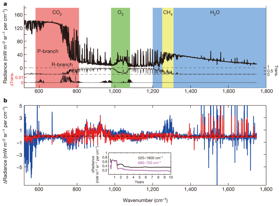
Figure 1 The top is what a spectrum looks like, with the radiance (think "brightness") at each different frequency (reported here as wavenumber). The left shaded red bit is mostly from CO2, and can be separated from the effect of other things like water vapour. The bottom shows, in red, the difference between the computer simulation and the measurements over March 2001. Differences in the CO2 region are mostly less than 0.5 units, out of total measurements of up to 140 units.
Some older studies that managed to measure over a longer period of time used instruments that weren't able to split up the atmosphere's spectrum: they could tell that more heat was coming down, but they couldn't directly measure the cause. Big, quick changes can happen because of changes in the air's temperature or the amount of water vapour, for example. These new measurements can tell the difference.
In the next step, the team calculated the amount of CO2-caused heating. They ran the impressively-accurate computer model LBLRTM with the observed changes in atmospheric temperature and everything else except for CO2. It was fixed at the starting level. Outside of the CO2 bands, the model matched the observations, but inside the CO2 bands the observations were different. This difference is due to the extra heat being sent down by CO2, and the team used this to calculate the growth in heating from CO2.
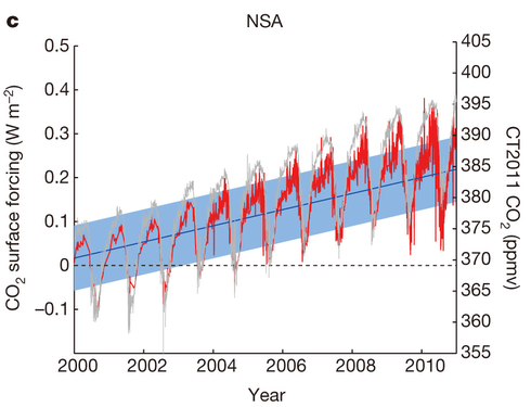
Figure 2 As measured at the North Slope Alaska (NSA) measurement site, the growth in CO2 heating effect is shown in red, and in grey the concentration of CO2 estimated to be in the bottom 2 km of the atmosphere is shown. The CO2 heating effect is in Watts per square metre, and the amount of CO2 in parts per million.
From 2000–2010, the CO2 we added to the atmosphere (22 parts per million) added another 0.2 Watts per square metre (W m-2) of heating to the surface. It was even possible to see the yearly cycle of plant growth: spring growth sucks up CO2 and reduces its heating effect, before the plants lose leaves for winter and the CO2 and its heating effect returns.
The extra heating reported here is not directly comparable with the effect known as radiative forcing, which is used to help project climate change. However, it confirms the calculations that have been used to work out these values.
Conclusions
We already knew that the greenhouse effect was real and that we're making it stronger. This new study uses some truly impressive measurements, and reports that they match the predictions of physics excellently. The computer models that apply these physics have been rigorously tested in the past and they are an amazing achievement.
I would interpret this study as being worth a sigh of relief: physics works great at calculating CO2's heating effect so we can move on to other problems. It's unlikely to change the opinions of those who deny the greenhouse effect though. Measurements showing that it exists and is getting stronger have been around for years, and evidence has failed to convince them so far, so there's no reason to think this will be any different.


Now prepare for the onslaught of flat-earthing pseudo physics that some will undoubtedly launch following these results...
Yep. The denialati were yelping about this paper last month (archived link). With the usual nonsense references to Salby, volcanos, "it's the sun", 2nd law of thermodynamics, etc...
Interestingly, this quote from the abstract:
And that the overall increase in the rates of warming being experienced by the planet (also called the Top of Atmosphere energy inbalance, or TOA) is growing at a much more rapid rate. This is especially true when one considers that the emissions of Chinese aerosols during this same period increased by over 400%
Thank you. One of my interests is amateur radio and I've been working with a fellow ham on IR cloudbounce communication. This is a nice lok at IR from another perspective. A very interesting article.
It's about time basic radiative forcing was validated 'in the wild'
Question - why doesn't the paper not compare measurement with theory? My back of envelope calc predicted 0.29 W/m2 vs measured 0.2W/m2.
5.35*ln(389.85/369.52) = 0.29 W/m2
Theo: I haven't looked into this, but the two obvious differences between this observation and a radiative forcing are that:
But there may be other differences.
Theo
you have an error of selection bias and improper time scales
The .2 value is a decadal average. You used a random start and end date instead of the annual average value and an 11 year time period.
Use the values from 2000 to 2010 and the points from the solid blue median line in the graphic.
Thanks for an excellent summary of an important new contribution.
I felt that one of the sentences in the article, "The extra heating reported here is not directly comparable with the effect known as radiative forcing, which is used to help project climate change," deserved further clarification. I think that this graph, taken from the IPCC AR5 WG1 final report (page 181) helps to explain the difference between the extra heating measured by Feldman et al. and the total radiative forcing used to project climate change:
Notice that the radiation "imbalance" (0.6 W/m2; lower left corner of the figure) is the very small difference between total incoming radiation and total outgoing radiation at the top of the atmosphere (TOA). This imbalance represents the "radiative forcing, which is used to help project climate change," and it is determined by interplay between many factors.
A large portion of the total heat radiation leaving the Earth's surface is returned to the Earth as "thermal, down surface" radiation (342 W/m2) by greenhouse gases and clouds (large orange downward arrow at lower right). Downward radiation from CO2 (as measured by Feldlman et al.) forms a significant component of that 342 W/m2, but downward radiation from water vapor and clouds is the major component according to my understanding. Downward radiation from CO2 is just one of the many factors affecting the final imbalance of 0.6 W/m2.
Fig 2 appears to be linear. Can a 100 yr projection be made to reduce impacts of internal variability forcing and accurately estimate temp increase given a consistent increase in CO2? Thx
Joel_Huberman @8, not quite right.
The energy imbalance at the top of atmosphere is composed of the change in radiative forcing minus the change in outgoing longwave radiation (OLR) due to the increased surface temperature. The total radiative forcing relative to 1750 in 2011 was 2.2 W/m^2, as shown by the IPCC AR5:
It follows that the OLR to space has increased 1.6 W/m^2. (Note, the imbalance at the TOA equals the imbalance at the surface to a very close approximation. If it did not, the atmosphere would heat, or cool very rapidly. The difference between that shown for the surface and TOA in your figure is entirely due to different rounding conventions.)
The radiative forcing, itself is the change in the downward energy balance at the tropopause after the stratosphere has reached radiative equilibrium (full IPCC AR5 definition at bottom of post). For convenience, we normally just refer to the Top of Atmosphere (TOA) rather than at the tropopause. That is reasonable because both are close approximations of each other.
Finally, the measured change discussed in the OP is in the "thermal down surface" shown in your diagram, as you correctly state. In the band of CO2 absorption, that change will have been due to increased CO2 concentration, increased H2O concentration and increased temperature. They appear to have determined the CO2 only contribution by comparision with a radiative transfer model (which unlike GCMs, are fully deterministic, and are very accurate). That change is small relative to the change in radiative forcing at the TOA, a fact which is well known. In fact, it is so well known that from time to time a denier will graph the expected changes at the bottom of the atmosphere as "proof" that radiative forcing from CO2 is much less than that expected by the IPCC - a proof that they are totally dishonest or hopelessly ignorant on the subject they purport to teach to others.
IPCC AR5 definition of Radiative Forcing (from WG1, Annex III)
Pblackmar @9, temperature increase at the surface due to radiative forcing is not a simple function of changes in back radiation (ie, the changes measured in this paper). That is because radiation is not the only energy transfer between the surface and atmosphere. Consequently, increases in back radiation may be matched by increases or decreases in convection, and or evapotranspiration. Rather, both changes in temperature, back radiation, convection and evapo-transpiration will occur to reestablish the change of temperature with altitude in the troposphere which enables an energy balance at the tropopause. Consequently the approach you mention will not reliably forecast future temperature changes.
Tom Curtis @10,11. Thanks for your excellent explanations. Clearly I had much to learn about how radiative forcings are calculated. May I ask you another question to test my new understanding?
Consider the first sentence of the IPCC definition of radiative forcing--"Radiative forcing is the change in the net, downward minus upward, radiative flux (expressed in W m–2) at the tropopause or top of atmosphere due to a change in an external driver of climate change, such as, for example, a change in the concentration of carbon dioxide or the output of the Sun." Based on the full definition and on your explanation, it now seems to me that the reason the measurements by Feldman et al. of changes in downward radiation due to changes in CO2 concentration do not correspond to radiative forcings is that these CO2-radiation changes may have induced other changes--changes in water vapor concentration or in cloud abundance, for example--which will also have effects on both upward and downward radiative fluxes at the TOA. Consequently, the net effect of a change in CO2 concentration will be composed of both a direct effect on CO2-radiation (downward and upward) plus indirect effects on other downward and upward heat transfer mechanisms. Feldman et al. measured a direct effect, but radiative forcing is the net effect. Is my current interpretation correct?
the 0.6 value of TOA is derived from Hansen and Sato (2010) and corresponds with an average value whose mid-point correltes with 2007. Recent NODC ocean heat content analysis shows that the TOA today is significantly higher and at ~1.0 Watts per meter squared in 2013.
It is plausible that, with significant reductions in SE asian aerosol emissions, we are currently at 1.2 Watts per meter squared and facing a significant rate of increase in coming years.
see: https://forum.arctic-sea-ice.net/index.php/topic,1183.0.html
Joel_Huberman @12, the definition, with my emphasis is:
Feldman et al measure the change at the bottom of the atmosphere, which they call the "surface radiative forcing". "Surface radiative forcing" and "radiative forcing" are not the same thing. For what it is worth, the change in downward flux at the surface due to a change in CO2, and absent any feedbacks, is about four fifths of the change in radiative forcing (as calculated by the IPCC approximation).
As you note, "surface radiative forcing" also differs from radiative forcing in allowing considerable atmospheric adjustment increase in CO2. That adjustment includes an increase in temperature and, importantly, an increase in H2O content. H2O absorption bands have considerable overlap with the main CO2 absorption bands. That is largely inconsequential for radiative forcing, for CO2 only decreases in concentration very slowly with altitude, whereas H2O is virtually absent above 3 km (except where there are very strong updrafts). Consequently, at the tropopause, the effect of H2O absorption in those bands is very small. In contrast, at the surface much of the effect of CO2 would occure regardless because of the presence of H2O. Further, the increase in temperature will increase the downward flux from all radiative components of the atmosphere including CO2.
It turns out the "surface radiative forcing" Feldman et al calculate is approximately equal to the radiative forcing as calculated for the TOA using the IPCC's approximate formula. As the change in net TOA flux allowing adjustments is considerably less than that, there must be some other difference in the surface energy budget making up the difference. To the extent that Feldman et al's results are respresentative of the global average, that difference will be made up by increased convection or evapo-transpiration, or heat flow from another region (or some combination of the three).
That response is a lot longer than needed as, except for specifying the difference in location (which you probably understood but thought too obvious to need stating), your understanding was correct. I just took the opportunity to flesh out some more of my thoughts on the topic :)
@tom 14
you said:
It turns out the "surface radiative forcing" Feldman et al calculate is approximately equal to the radiative forcing as calculated for the TOA using the IPCC's approximate formula.
I have reviewed the paper and supplemental information and have not found an absolute value for surface radiative forcing that is equal or approximate to TOA values. Do you have a value or quote from the paper that justifies your statement? What is the Feldman total surface radiative forcing in their series at 2007?
The references show that the total longwave downwelling trend is 2.1 watts per meter per decade increase.
jja @15, eyeballing figure 2, CO2 concentrations at North Slope Alaska have grown from 369-385 ppmv, for a calculated increase of 0.227 W/m^2 of forcing, which is approximately the same as the 0.2 W/m^2 increase in surface radiative forcing shown on the trend line (blue).
However, as you challenged the value, I looked at global annual average increases in CO2 from 2000-2010 (368.85-388.57 ppmv) for a global increase of forcing of 0.279 W/m^2. Further, the calculated forcing for the annual average increase for Alert, Alaska (data), is 0.277 W/m^2 . These are not approximately 0.2. Further, the standard formula for radiative forcing of CO2 applies only to global values, and not necessarilly for regional values. Consequently I withdraw my claim.
I will note that using Modtran and the Alert values with the standard cirrus model, there is a 0.09 W/m^2 TOA difference in radiative flux for the sub-arctic summer and winter. On that basis, the standard formula radically over estimates TOA radiative forcing of CO2 in the sub-arctic (including Alaska). Of course, the modtran model at UChicago is obsolete, and I did not set up the model properly to get the change in radiative flux at the tropopause, after the stratosphere had adjusted nor to get all sky values, so the modtran estimate of forcing is very approximate.
Tom
the 0.2 watts per meter squared increase per decade is a good fit for the TOA analysis using Nuccitelli et al 2012 with Durack 2014 reanalysis. However this is a decadal rate of change, not an absolute value.
The absolute value was estimated by Hansen and Sato (2010) using Levitus et. al (2009) data at 0.6 watts per meter squared, corresponding to a median date of 2007.
However, recent NODC 0-2000 meter OHC analysis shows that the lower bound of current TOA radiation imbalance is 1.0 Watts per meter squared. This is a least bound as the rate of TOA is currently increasing and increasing at an increasing rate!
it was your use of the term TOA that threw me off. I have not seen a good analysis of TOA time series except for the one that I have done as an amateur compilation.
jja @17, Feldman et al measured the surface radiative forcing of CO2. The total surface radiative forcing will have been larger than that. Therefore, for comparison I compared it with the radiative forcing of CO2. The net TOA energy flux that you discuss includes the total forcing since 1750 from all sources, minus the increase in net upward energy flux due to increases in GMST including feedbacks on that temperature increase.
Theo @5:
Quick answer is: they did compare measurements to theory and found the model did excellently, see Figure 1 in the paper.
Your equation is an approximation from Myhre et al. (1998). It's for net change in flux at the tropopause after allowing the stratosphere to adjust, and averaged over 3 different atmospheres (tropical, northern and southern).
This experiment has measurements from two land surface locations, both Northern Hemisphere, only clear-sky and including changes in temperature and water vapour.
Since CO2 and water vapour have some absorption band overlap, then they each steal some heating from the other. So if you increase CO2 without increasing water vapour (like in Myhre et al) then the calculated CO2 effect should be bigger than the case where water vapour increases (like in this experiment). That's just one reason why we should be careful with the comparison.
Both Myhre et al. and this study use line-by-line models that are astonishingly accurate (e.g. Tjemkes et al., 2003). These new measurements gives us even more confidence that these models can be used to estimate radiative forcing.
We'd already checked these models "in the wild", and satellite measurements also back up expected changes (e.g. Harries et al., 2001). This new study seems to be built on a top quality experiment, but we already had enough experimental evidence to be very confident in the radiative transfer models used to calculate radiative forcing.
jja @17:
Is this the sort of thing you've been looking for? We now have estimates of the TOA imbalance in each decade.
MarkR @20 Allen et. al. 2014 is included in the graphic. The error bars make it practically worthless compared to hansen and sato 2010, though it does give a higher mean value as shown on the graphic above.
MarkR,
I'm hoping you can help clarify something for me. Jim Steele makes a novel suggestion regarding Heat Waves. It seems wrong on a number of levels, but I sure can't put it together into words. I'm hoping you can help, here's the quote:
citizenschallenge:
I don't have a cite, but to the best of my knowledge:
(1) A heat wave does not require the absence of atmospheric water vapour, or indeed of water stored in soil, etc.. IMO your interlocutor needs to provide a cite to support the claim "heat waves usually occur under very dry conditions". (Obviously not a veteran of Ottawa, Ontario heat waves, then.)
(2) Atmospheric water vapour is geographically and temporally highly variable (e.g. there is less of it in, say, desert regions, or in polar regions during the winter, than, say the wet tropics).
I can't say I know much about heat wave formation, but I'm rather doubting the person you are quoting does, either.
RE: citizenschallenge #22
Please correct me if I'm wrong: It is my understanding that heat waves (high pressure domes) are a consequence of wind patterns (or lack there of), primarily. So both the start of a heat wave, and its ultimate conclusion, are at the hands of a much larger-scale planetary wind/ocean currents.
The idea that "local" humidity effects the duration/severity of heat waves seems a bit like a "forest for the trees" type of error - to me. It makes sense that local humidity is important - but not really THAT important.
If any one can clarify...
Citizenschallenge,
As I understand it Jim Steele has it almost backwards. AGW causes dry places to get dryer. Heat waves are worse when there is little surface water to evaporate and cool the atmosphere. In places like California, they have had little rain. When they have a heat wave, it is much hotter than it would have been because there is no water to evaporate to cool the weather off.
AGW's twin effects of altering rainfall and making it hotter causes heat waves to be even more distructive. California has had its fourth dry rainy season. It has been record hot there for months. Expect this summer to be even hotter and have a worse fire season (another of the effects of AGW). They pray El Nino will bail them out but no luck so far on that.
Link to Tjemkes et.al 2004 is broken.
Nature has changed its link. The Feldman article is no longer at the listed
http://www.nature.com/nature/journal/vaop/ncurrent/full/nature14240.html
It is now at
https://www.nature.com/articles/nature14240
Now "Nature" has put the article back behind a paywall.
If there were anything more perverse in the world than the way they attempt to make money by "owning" knowledge, I never heard of it.
[DB] A direct link to a full copy is here and also here.
Thanks for that. Link in the article needs to be fixed too though.
regards BJ