


 Arguments


2015 SkS Weekly Digest #27
Posted on 5 July 2015 by John Hartz
SkS Highlights
Pope Francis’ call for urgent action to combat climate change has generated unprcedented news coverage and discussion throughout the world over the past few weeks. It is therefore not surprising that the 2015 SkS News Bulletin #6: Pope Francis & Climate Change garnered the highest number of comments of the items posted on SkS during the past week.
El Niño Impacts
- Peru declares emergency in 14 regions on El Nino worries by Mitra Taj, Reuters, July 5, 2015
- El Nino to Weaken Monsoon, Exacerbate Drought in Pakistan, Northwestern India by Alex Sosnowski, AccuWeather, July 4, 2015
- Strengthening El Nino Possibly Linked To More Shark, Exotic Fish Sightings Off California Coast by Nicole Jones, CBS SF Bay Area, July 2, 2015
Toon of the Week

Hat tip to I Heart Climate Scientists
Quote of the Week
"In Dante's Inferno, he describes the nine circles of Hell, each dedicated to different sorts of sinners, with the outermost being occupied by those who didn't know any better, and the innermost reserved for the most treacherous offenders. I wonder where in the nine circles Dante would place all of us who are borrowing against this Earth in the name of economic growth, accumulating an environmental debt by burning fossil fuels, the consequences of which will be left for our children and grandchildren to bear? Let's act now, to save the next generations from the consequences of the beyond-two-degree inferno."
The beyond-two-degree inferno, Editorial by Marcia McNutt, Science, July 3, 2015
SkS in the News
The TCP is prominently referecned in:
- STUDY: How The Media Is Covering Presidential Candidates' Climate Science Denial by Kevikn Kalhoeffer, Media Matters for America, July 1, 2015
- When politicians talk science by Stephen H. Jenkins. OUPblog, June 28, 2015
- The Pope's Ecological Vow by Paul Vallely, New York Times, June 28, 2015
SkS Spotlights
The mission of the Cambridge Institute for Sustainability Leadership (CISL) is to empower individuals and organisations to take leadership to tackle critical global challenges.
We are an institution within the University of Cambridge
Across complex and connected issues, we challenge, inform and support leaders from business and policy to deliver change towards sustainability.
We help influential individuals, major organisations and whole sectors develop strategies that reconcile profitability and sustainability and to work collaboratively with their peers not only to develop solutions to shared challenges but also catalyse real systems change.
Our work
For over 25 years we have been working to build leadership capacity to tackle critical global challenges, through our business action, executive education and Master's-level programmes.
International locations
We have offices in Cambridge, Brussels and Cape Town, and delivery partners in Beijing, Melbourne and São Paolo.
Working with multinational businesses, multilateral agencies and national governments, we deliver projects on the ground in Europe, Africa, North and South America, Asia and Australia.
We have a strategic focus on extending our work with business and governments in China and Brazil, and across Africa.
Coming Soon on SkS
- Announcing the Uncertainty Handbook (Adam Corner)
- Carbon cycle feedbacks and the worst-case greenhouse gas pathway (Andy Skuce)
- Climate denial linked to conspiratorial thinking in new study (Dana)
- 2015 SkS Weekly News Roundup #28A (John H)
- Who knows what about the polar regions? Polar facts in the age of polarization (Lawrence Hamilton)
- Dutch government ordered to cut carbon emissions in landmark ruling (Arthur Neslen)
- 2015 SkS Weekly News Roundup #28B (John H)
- 2015 SkS Weekly Digest #28 (John H)
Poster of the Week
SkS Week in Review
- 2015 SkS Weekly News Roundup #27B by John Hartz
- More evidence that global warming is intensifying extreme weather by John Abraham
- New study warns of dangerous climate change risks to the Earth’s oceans by Dana
- 2015 SkS News Bulletin #6: Pope Francis & Climate Change by John Hartz
- 2015 SkS Weekly News Roundup #27A by John Hartz
- As the Denial101x course ends, a new one begins by BaerbelW
- A Southern Hemisphere Booster of Super El Niño by Rob Painting
- Irreversible loss of world's ice cover should spur leaders into action, say scientists by Roz Pidcock (The Carbon Brief)
- 2015 SkS Weekly Digest #26 by John Hartz
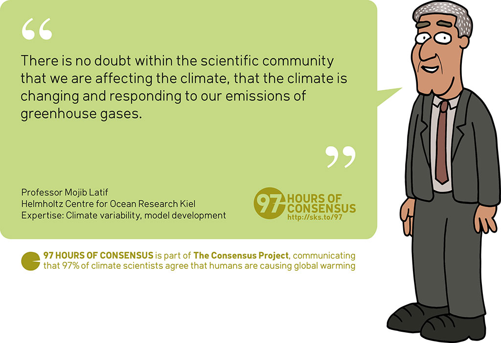
97 Hours of Consensus: Mojib Latif


Only just noticed the "Coal-Fired Mercury Polluton" on the industrialist, so I guess that makes it 20% envionmental 80% unhelpfully divisive (5 separate issues presented). My point stands though, if I as a progressive reader misunderstood the context, then what is a conservative reader to make of it?
[JH] My apologies to you for accidentallly deleting your prior comment. I will repost the text.
I think you have a point.
I accidentally deleted the following comment. My apologies to macoles.
macoles at 14:46 PM on 7 July 2015
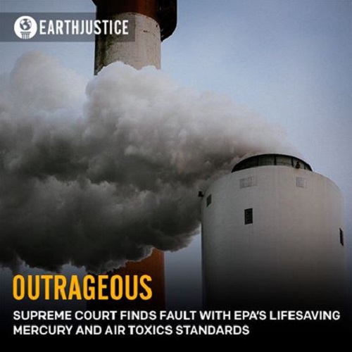
Am I the only one here who thinks the toon of the week above is 0% climate science 100% unhelpfully divisive?
Yes conservatives can get some dreadful things through the supreme court (poster of the week above for example), but whether we like it or not getting them on board is a big part of the solution. Gay marriage only just passed 5-4 because one normally conservative judge was able to be convinced.
Lampooning conservative bad liberal good on a respectible site like this only plays into the hands of those who think climate change is some ideological hoax.
Macoles:
You have a point. I will be more judicious when selecting future Toons of the Week.
I somewhat disagree. Within the 'conservative' camp you've got people who will never break from tribalism, people who might (those you are concerned about alienating), and people who don't even realize what their side is really doing. (Ditto liberals/progressives, though the percentages are different).
The cartoon above is beneficial for educating that last group. Whether that outweighs the potential harm of alienating some portion of the middle group is hard to say, but I'd argue that both are fairly small in comparison to the bloc that won't change until their 'leaders' tell them that they believed differently all along.
[JH] Thank you.
Perhaps you are right CBDunkerson, but one of the things that makes this site unique from many other pro-science sites is it strives to explain the science while trying to keep the usual argy-bargy at arms length. When we provide links to articles here from conservative forums we know we won't convince the unconvincable, but we do hope others will follow and find their assumptions challenged. The toon of the week seemed to me to only reinforce conservative assumptions.
Michael FitzGerald @here.
You say @that3 "Your equation seems to assume that dT/dF is linear" but my equation is dT/dF = 0.25 x 65 x F^-0.75. How can that be linear?
Michael Fitzgerald from elsewhere asks "...what is the sensitivity as a function of temperature?"
The simplest response is that the sensivitity function is given by the Stephan-Boltzmann law, j* = σ * T4, where j* is the power in Watts per meter squared, σ is the Stefan Boltzmann constant, and T is the temperature, in this case the Global Mean Surface Temperature (GMST).
Transforming the equation to a formula for temperature, we have:
1) GMST = (j*/σ)^0.25
j* in turn is the sum of the effect of all forcings and all feedbacks. That is, it is the globally averaged insolation, times (1 - albedo) plus the total greenhouse effect. Putting those numbers in we have
GMST = ((0.25 * 1360 * (1 - 0.3) + 150)/σ)^0.25 = 287.6 K, or 14.46 C
Very clearly this is an approximation as I have ignored emissivity, which raises the temperature in degrees K by a degree or so (as the Earth is not a perfect black body at IR temperatures), and the uneven distribution of surface temperatures (which would lower it by approximately the same amount), but it is a pretty good estimate, as can be seen by comparison with the estimates from observations (14 C from HadCRUT4, 13.4 from GISSTEMP) and from models (CMIP5 mean of 13.7 C) which take far more detail into account (right section of graphs).
Using all known energy sources for the Earth's surface and the current total greenhouse effect (rather than that from the 1980's as used in the calculation above), the estimate absolute temperature using this formula comes out at 289.65 K, but again given the approximations involved that is quite good.
From your discussion with MA Rodger, it appears that you may be confusing the result of this equation with the Climate Sensitivity Factor, λ, which is defined such that the temperature response to a given forcing (ie, not including feedbacks) that perturbs the Earth's temperature from a prior quasi-equilibrium is:
2) ΔT = λ * ΔF
where ΔT is the change in temperature, λ is the climate sensitivity factor (having units of degrees C per W/m^2) ΔF is the change in forcing. This works as a linear approximation only for small perturbations relative to the total incoming energy plus total greenhouse effect. Further, it only works for conditions approximately like those currently existing. Clearly at very low temperatures λ would be much different from current values both because of the larger planck response to temperature (ie, the response based on the Stefan-Boltzmann law), and because many feedbacks that currently exist would not exist, or be very much weaker. For example, much below the freezing point of water there is no water vapour feedback and essentially no albedo feedback. More than a hundred degrees below the freezing point of water and there is essentially no greenhouse effect (because all of the CO2 would have precipitated out of the atmosphere), and so on. It follows that it is a mistake to try and apply formula (2) except in current conditions. However, in current conditions, λ is for all intents and purposes the "sensitivity as a function of temperature", and is approximately 0.75 which corresponds to a climate sensitivity of 2.8 C per doubling of CO2.
MA Rodger @7, you appear to have taken the derivative of formula (1) @8, which gives (if I have done this correctly):
(3) dT/dF = 1/σ*0.25*(j*/σ)^-0.75
However, you express the relationship between σ and j* as a product rather than a ratio, and I am not sure how you derive the value 65 in your concluding sum which eliminates σ from the calculation. Could you clarrify.
OK. But isn't ΔT/ΔF (λ) just the slope of the Stefan-Boltzmann relation at 255K? In your calculation, you added 150 W/m^2 of extra warming power to the 238 W/m^2 of solar power (255K). That being said, increasing 238 W/m^2 to 239 W/m^2 should only result in another 0.63 W/m^2 to the 150 W/m^2 of warming resulting in a surface temperature of 287.9 K which is 0.3C warmer, or 0.3C per W/m^2 and not 0.75C per W/m^2. Where does the extra 0.45C come from?
Michael Fitzgerald @10, the slope of the Stefan-Boltzmann function at 250 W/m^2 is 0.258 Degrees K per Watt/m^2. At 400 it is 0.181 Degrees K per Watt/m^2. Neither is λ. That is because λ includes not only the planck response (ie, the slope of the Stefan-Boltzmann function) but also the further effect of any feedbacks. These increase the temperature response by 1.5 to 4.5 times the base response, ie, increase λ to 0.39 to 1.16 K/W/m^2.
I used the value of the Planck responce at 250 W/m^2 for that calculation because forcings are calculated for the TOA (ie, near to the effective altitude of radiation to space where the temperature calculation does not include the greenhouse effect), and hence λ is defined for that altitude as well. We could calculate a climate sensitivity parameter for surface forcings but the values would differ from the more conventional calculation for the TOA.
It is at 238 W/m^2 which corresponds to the 255K temperature of the planet from space. 238 W/m^2 -> 254.53 and 239 W/m^2 -> 254.8K for a difference of 0.28K per W/m^2. If I do the other calculation to 2 decimal places (instead of 1) I also get 0.28K per W/m^2. One W/m^2 of forcing from the Sun after reflection is the same at all altitudes from TOT to TOA so why is there any distinction (You said forcing is defined at TOA, but I thinkj you meant TOT)? The input power is still 239 W/m^2 (up from 238 W/m^2) and the sensitiivty is defined to be relative to this difference. I don't see how the temperture at TOT is relevant. The temperature at TOA is 255K.
Also, isn't the current surface temperature consequential to 238 W/m^2 of input and that 150 W/m^2 of additional warming power already the LTE (i.e. after all feedback has been accounted for) result? What additional feedback can make that much difference?
[PS] A quick look at the IPCC Technical Summary, especially TFE.6, pg 82 might help getting you on the same page with respect to definitions etc.
Moderator,
The page you pointed me to was all the uncertainties. The other page 82 is a different document. Anyway, in the document you refered me to radiative forcing was defined as,
Radiative forcing (RF) is a measure of the net change in the energy balance of the Earth system in response to some external
perturbation. It is expressed in watts per square
metre (W m–2); see Box TS.2
Box TS.2 on page 53 defines it more precisely as a net difference at the top of the troposphere after the stratosphere has arrived at equilibrium but keeping all other state, including surface temperature, constant.
Thanks for the reference.
Michael Fitzgerald @12 and 13, what you call TOT (Top of Troposphere) is by convention called Top of Atmosphere (TOA) by climate scientists. The IPCC Annexe III for WG1 says:
As you can see, " top of atmosphere" is given as an alternative term for the tropopause (by definition the top of the troposhere). The reason for this convention is probably partly historical and partly convenience. As to convenience, the difference between radiative fluxes at the top of the troposphere and at the (very ill defined) highest altitude with gaseous content is small, as you note yourself, so that the convention make little difference in the approximate estimates in which it is used. Historically, early climate models did not include a stratosphere, so that the Top of Model (the other term you will see) was also the tropopause), which I presume helped give rise to the convention.
If you want to discuss the literal top of the atmosphere, we face a problem that it is undefined. The Karman line is, by convention, the demarcation between the "atmosphere" and "outerspace", but it demarcates the lowest levels of the thermosphere as being in the atmosphere, while the bulk of the thermosphere is treated as being in outerspace. Ergo it is an entirely arbitrary demarcation with no physical basis. Worse, the particles in the thermosphere still act as a gas meaning that however tenuous, they are an atmosphere. Further, the thermosphere is radiatively significant (although almost inconsequential as regards surface temperatures).
Moving on, the temperature at the top of the gaseous envelope of the Earth is not 255 K. Depending on whether you define it as the Stratopause, Mesopause, Karman line, or Thermopause it is approximately 275 K, 180K, 220 K, or much greater than 270 K.
Where the temperature is 255 K (ignoring temporal and geographic variation) is the average altitude of radiation to space, also known as the skin layer. This can be treated withto a reasonable approximation as the altitude within the troposphere whose temperature matches that of the skin layer, or about 5 km above the surface.
Finally, the advantage of using the tropopause to define radiative forcing is that the temperature at the tropopause is fixed relative to the surface by the lapse rate induced by convection. That means that temperature changes in the tropopause are more or less constant with altitude, ie, a 3 C increase in temperature at the tropopause will result in a 3 C increase at the surface, and vise versa. This again is only true averaged across the diurnal and seasonal cycle, and ignores the effects of the increase of altitude of the tropopause with increased global warming, and the lapse rate feedback (ie, the cause of the tropospheric hotspot). This relationship of equivalent temperature changes allows you to reason out the effects of radiative forcing without needing always to use a full GCM (which is the only way to avoid such rule of thumb reasoning).
There is definitely some surface of some radius where radiative fluxes are in balance. The specific temperature of rarified upper atmosphere gases shouldn't be very important as their specific emissivity is so close to zero they contribute little to the flux of photons leaving the planet. We should be able to define some radius where the net flux of photons is on average zero, beyond which power emissions drop off as 1/r^2. From space, this radiation is directly measured by weather satellites whose LWIR senors see surface emissions and see cloud emissions but do not see LWIR emissions from anything above the troposphere except perhaps buried in the noise.
You are saying that this boundary is about 5 km above the surface. This seems to low to me since clouds can extend to the top of the troposphere and the coldest cloud tops are about 260K. 5 km above the top of the troposphere seems more plausible. Anyway, getting late here, will pick this up again tomorrow.
Thanks for your time,
Michael
Tom Curtis @9,
The 65 is an approximation of σ-¼ = 64.8.
j*=σT4
T = σ-¼ x j*¼= 64.8 j*¼
dj*/dT = ¼ x 64.8 j*-¾
This gives the slope of the Stephan-Boltzmann equation which at j* = 238.5 Wm-2 yields a slope of 0.2669444ºC/Wm-2. The approach employed @12 by Michael Fitzgerald gives a slope of 0.2669446 ºC/Wm-2. As the concept of climate sensitivity compares ΔT resulting from a doubling of CO2 where ΔF = 3.7 Wm-2, zero-feedback sensitivity = 0.267 x 3.7 = 0.99ºC which happily is the value quoted in climatology and Wikipedia.
[PS] Well yes, but a very carefully worded restatement could be - ie something like how much extra temperature change would there be for a purely forced temperature change of 1 degree. It still comes down to magnitude of feedbacks - and also timeframe of interest since have both fast and slow feedbacks.
MA Rodger @16, thankyou.
MIchael Fitzgerald - Keep in mind that satellites are not looking at a single emitting layer at a single temperature, but rather a range of wave-length dependent radiating altitudes where given the GHG spectra the majority of emissions can reach space. I've commented previously on this topic here.
Secondly, it's entirely clear to me whether you're accounting for the lapse rate between the effective emission altitude and the surface - the Stephan-Boltzmann dependent emissions from TOA are in essence amplified by the lapse rate to actual surface changes.
Once again we are reminded that science is a never-ending process...
New technique for analysing satellite data will allow scientists to predict more accurately how much the Earth will warm as a result of carbon dioxide emissions.
Quantum leap taken in measuring greenhouse effect by Tim Radford, Climate News Network, July 8, 2015
KR,
Yes, the satellites have sensors that span wavelengths. Most have one or 2 bands covering the transparent window(s) on either side of the 10u ozone lines, a sensor tuned to a specific water vapor absorption line for detecting atmospheric water content and newer satellite often have a NIR band which is useful for detecting nightime differences between clouds and surface ice/snow which is important at the poles when its dark for half of the year.
Other than the water vapor channel, little energy in GHG absorption bands is detected by these sensors, except perphaps at the edges, as they as specifically tuned to avoid them, not because of the lack of emissions in those bands, but because the attenuated emissions in those bands makes backing out the temperature resulting in those emissions more difficult. There's also some parallax processing you can do with multiple images from one or more satellites in different places to distinguish the specific height from where radiation originates, specifically when images from different geosynchronous satellites overlap. Something similar is done to produce 'helicopter' imagery for Google, Apple and Bing maps.
We seem to be getting a little OT here. My original question was about the sensitivity as a function of temperature so that we can slowly ramp the accumulated forcing from 0 to 239 W/m^2, sum up the effect from each incremental W/m^2 and arrive at the correct surface temperature. This relationship may not be known, but based on what has been said so far, we can create a template for it must look like. We know this is not a linear relationship and can't even be monotonic. Earlier you said that that below about 173K there's no GHG effect (and no clouds either) and the reasons certainly make sense, thus the first 51 W/m^2 of accumulated solar forcing offsets the emissions at 173K where the slope of the Stefan-Boltzmann relationship at 173K is about 0.85C per W/m^2. If the sensitivity to forcing thereafter slowly ramped down to 0.75 C per W/m^2 at 239 W/m^2 of accumulated forcing for an average sensitivity of of 0.8C per W/m^2, the final temperature would be 173 + (239-51)*0.8 = 323K which is way too high, thus the sensitivity must drop well below 0.75 eventually rising to 0.75C per W/m^2 at 239 W/m^2 of accumulated forcing. This contradicts other evidence that suggests the GHG effect gets larger as you get closer to the poles implying a higher sensitivity at colder temperatures and the reason for my concern. This behavior makes sense because each incremental degree of surface temperature requires more accumulated forcing to offset the increase in Planck emissions and the sensitivity should decrease as temperature increase unless positive feedback also increases as the temperature rises.
Michael
Michael Fitzgerald @15, as the planetary energy budget is not currently balanced (as a consequence of which we are warming), there is no current boundary across which the energy flows are in balance. Indeed, as peak warmth or cold either seasonally or diurnally does not coincide with peak radiative flux (due to thermal inertia), there is never such a boundary except as a transitory state. That is why the climate is considered to be in quasi-equilibrium when it reaches the nearest approximation to an equilibrium state.
More directly, in this calculation we are attempting to balance (or nearly balance) the OLR with the annual average insolation. As such, we are also using the annual average OLR. That clouds occasionally have tops higher than approx 5 km at given locations does not mean the globally and annually averaged radiation to space does not have an effective altitude of radiation to space of 5 km. If you want to take into account specific weather patterns, and the diurnal cycle etc, you need a GCM, not the simple formulas we are discussing.
Finally, you are ignoring the fact that CO2 (and methane and ozone etc) only absorb IR radiation at specific frequencies. At some frequencies, the radiation to space actually comes from the surface (unless clouds intervene). At other frequencies, it is radiated by H2O in the atmosphere, and typically comes from 2-3 km from the surface. At other frequencies it is radiated by CO2 and comes from virtually at the tropopause. Averaged across all frequencies it effectively radiates from approximately 5 km altitude.
Michael Fitzgerald @21, some statellite instruments are tuned to frequencies to avoid CO2 and H2O absorption bands. Other instruments cover a wide range of frequencies:
FYI, the approximate altitude of emission at a given wavenumber can generally be determined using the temperature of the ground (approximately given at 900 cm^-1) and the lapse rate. That is difficult for the spectrum over Antarctica (in which there is a strong temperature inversion resulting in CO2 warming the surface, unlike the usual condition) and for the spikes at the center of the CO2 band (667 cm^-1) and the ozone band (approximately 1050 cm^-1), both of which represent radiation from the stratosphere.
Michael Fitzgerald @22:
I have it from reliable authority (Chris Colose) that the greenhouse effect increases more rapidly in the tropics. This would prevent the escape of heat, forcing a larger energy flow from equator to poles, thereby warming the poles. Polar amplification would constitute a combination of this effect, the smaller enhancement of the polar greenhouse effect, and the reduction in polar albedo.
You are ignoring the fact that atmospheric water vapour increases with the fourth power of SST. That strongly suggests an increasing climate sensitivity parameter with temperature, particularly once polar ice becomes negligible. In fact, the to most important factors governing the changes of the value of λ with temperature are the latitude of polar ice (the lower the latitude, the higher the sensivity) and the amount of evaporation (with higher temperatures indicating higher senisitivity). That suggests we are currently near the bottom of a trough in the value of λ, with any increase in temperature sufficient to eliminate arctic sea ice sufficient to put us onto an increasing λ with temperature, if we are not already past the inflection point.
Tom, re24.
Yes, this is spectrum I expect. The emissions in the absorption bands are about 1/2 of what they would be without GHG absorption (a little less at 15u where there is significant overlap between CO2 and H2O) when compared to the transparent regions whose Planck shape is approximately representative of the surface temperature for the Sahara and Med measurements. The Planck shape of the Arctic measurement is too low to be representative of the surface temperature and is likely a measurement of cloud tops which exhibit little GHG effect to space due to almost no water vapor and little atmosphere to begin with. Inversions generally don't have anything to do with CO2 and are when cold air sinks into valleys and the surrounding high ground become warmer. It looks to me like the spectrum from a cloud covered Antarctic mid winter. Do you know the time of year this was measured?
Ok, less emisions from absorption bands increases the sensitivity as the temperature increases. Is this enough to overcome the T^4 increase required to sustain higher temperatures? The T^4 difference between the emissions at the Med temp of 285K and the Sahara temp of 320K is almost a 60%. The plots don't seem to show enough incremental GHG effect to offset this much incremental power and then some to achieve a net increase in sensitivity. Is this difference quantified anywhere?
It's hard to tell since viewing this as linear wavenumbers isn't the most representative of where the power is. Plotting with an X axis of log wavelength or log wavenumber give a better perspective on where the power densiity is. Note that while frequency/wavenum plots have the peak near wavenumber of 700, the peak of the Planck distribution by wavelength is closer to 10u (wavenum=1000). The shapes of these curves makes a big difference in perspective relative to the strength of the lines. You should try different X scaling when plotting MODTRAN generated spectra and see what happens. I suspect an accurate visualiation of the power density is somewhere between the two.
Tom RE 23.
The Earth is hardly ever in transient balance because the seasonal solar input per hemisphere varies faster than the system can adapt. As seasonal solar peaks and starts to fall, it continues to warm until the input power drops below the value required to sustain the current average and then the temperature starts to drop. The inverse of this happens past the minimum seasonal input. Min/max average temperatures then lag min/max seasonal solar input by about two months. The solar input and planet output emissions cross each other twice per year, around Mar and Sept where the system is transiently in balance. If this difference is integrated over an entire year, the result should be very close to zero, although I suspect it varies some on either side. The record also shows year to year differences in average temperature of up to 1C both up and down, so if the planet average can move 1C or more in a year whether by changes in solar input or changes in state, whatever effect past CO2 emissions might have should have mostly been manifested. The exception being some fraction of emissions over the last year or two, so its hard to imagine much unrealized effect.
A question for you is if we specify a Gaussian surface surrounding the Earth, measure the energy flux of photons passing in both directions acriss this surface and average this over a few decades. or even a single year, what would the average flux be? Its easier to think about when energy is only flowing in one direction, for example from Earth to space, where we could consider the Earth an antenna radiating LWIR and the power passing through this Gaussian surface will always be the power driving the antenna which in this case is the power radiated by the planet.
Another think I was thinking is relative to the 150 W/m^2 of extra warming added to the 239 W/m^2. If the 150 W/m^2 increases linearly with forcing, then delta T / delta P is the slope of SB at 255K or about 0.3C per W/m^2. To get the required 0.8C from 1 W/m^2 of forcing, we need the 150 W/m^2 of extra warming to increase by 3.3 W/m^2, rather than the 0.6 W/m^2 when each W/m^2 of input contributes equally to the 150. This results in a GMST of 288.4K which is the required 0.8C larger then the original 287.6K. I just don't know how to justify the 3.3 W/m^2 instead of 0.6 W/m^2 as the increase in excess warming power.
FYI, I will be taking tomorrow off and heading to the mountains for some back packing. I will be back late Sunday and can continue the thread after work on Monday.
Thanks,
Michael
Michael Fitzgerald @26, not in order:
1)
The units of the y-axis in this plot are microWatts per meter squared per steradian per line number {mW m^-2 Sr^-1 (cm ^-1)^-1}. Multiply by a suitable constant and that becomes microWatts per meter squared per cm^-1. Put simply, it graphs power output per unit area linearly against line number. The equivalent plots against wavelength have a different shape because line number is an inverse function of wave length. Ergo they are not one to one. They are both accurate, and both accurately represent where most of the power is radiated (relative to the respective units).
2) There is no plot above for Arctic conditions, only for Antarctic conditions where surface temperatures do fall below 193 K in winter. Ergo it is very likely that the Antarctic spectrum represents the (near) blackbody spectrum of the surface with humps from warmer CO2 and O3 due to a temperature inversion (common in Antarctic winters). If the low temperature were due to high cloud cover, the brightness temperature would be near constant across the entire spectrum.
3) It is a mistake to compare the difference in surface emission (ie, the black body radiation for the surface temperature) in comparing different conditions. By definition, the surface radiation excludes any greenhouse effect, and therefore cannot show the effect of the water vapour feedback. Nor can you sensibly determine the strength of the water vapour feedback by comparing to Sahara conditions, ie, conditions with virtually zero water vapour due to being below the downwelling of a hadley cell. More appropriate is a comparison between mediterrainian conditions and those over the Niger Valley:
Michael Fitzgerald @27.
I do wonder reading this comment. Even as I pack away my woolly bobble hat and hang up my straw panama beside the front door, it is blatantly evident to anyone familiar with AGW that there is an imbalance between the Earth's incoming and outgoing radiation and has been for some decades. It is of truly massive proportions, enough to elevate global average surface temperature by 0.3ºC annually, 3ºC decadally, but because the Earth comes equipped with a giant heat sink attached, the impact of this massive imbalance is far smaller. This heat sink is known technically (and commonly so you will have heard of it) as "the oceans" and it is the rise in ocean heat content that allows climatology to be confident about the size of the imbalance.
So I do wonder. Would it be more sensible with this discussion to set out what is being discussed. The concept of ECS and its application in quantifying the impact of all types of climate forcing - this concept only works usefully over small variation in temperature. (This has been said above.) If, Michael Fitzgerald, you wish to expand the scope of the ECS concept in more than a trivial way, the concept needs redefining. Otherwise your discussion here, as conducted by you, is taking the michael out of those who are contributing in good faith.
MIchael Fitzgerald - Comments, not in any particular order.
Overall, I have the impression that you are getting lost in the minutia, and trying to extrapolate from those to global conditions. Beware the fallacy of composition.
I have time for one comment before I disconnect from technology for a few days.
A heat sink seems to be the wrong term. A heat sink redistributes heat. Consider the heat sink in your computer. When you turn your computer off, it starts to cool immediately. If what you are saying is true and the Sun stopped shinning (technical details of this aside ...), the Earth would continue to warm for centuries. It seems to me that if the Sun stopped shining, Earth would become an frozen wasteland in a matter of weeks.
Since the start of the industrial revolution, man has gotten about half way to the doubling CO2, meaning that since then, GHG forcing consequential to mans CO2 emissions has increased by about 1.7 W/m^2. To suggest that the planet hasn't been able to adapt to this doesn't seem logical, especially considering how quickly the planet adapts to seasonal variability.
The concept of missing heat presumes a high sensitivity. If the sensitivity was much less than 0.8 C per W/m^2 wouldn't that be an equally valid explanation for the apparent missing heat? How can we tell which is the right explanation?
Michael Fitzgerald @32.
Well bless by straw panama hat. Is the sun likely to stop shining?
The heat sink in my computer sucks energy away and out from the machine preventing it from overheating in its steady state working condition. In that respect, the oceans are not a good analogy as at steady state the climate system is in equilibrium with the oceans. But in a warming climate, which is the present state the climate, the oceans do provide cooling, preventing the surface from reaching any equilibrium temperature for many decades. In that respect, they are a heat sink and the increasing OHC is conclusive evidence of that warming climate. You seem reluctant to accept this truth.
Further, you seem to want to trivialise AGW because the temperature variability of the seasons is so much greater. You introduce here something you term "the concept of missing heat" but you fail to explain the concept. It appears to be some grand theory as "equally valid" as AGW. So do please explain where climatology has been going wrong all these years. I'm sure we will find it most entertaining.
Moderator.,
My last post seemed to have dissappeared. I can repost it if necessary.
Michael
[PS] It appears it was deleted for sloganeering (not me). Try again without the preamble. I would also suggest that since you are proposing sensitivity might be low, that an appropriate place to post would "Climate sensitivity is low". (be sure to read the article). To answer the question as to whether climate might be sensitive enough to be damaging, then you need to look at ECS not just the instantaneous change.
I'll remove the response to MA's comment from the preamble, as his comment about evidence of warming was OT anyway.
I also think that this is the more relevant thread, as I'm not claiming any specific sensitivity, high or low, and am just characterizing a test of the sensitivity.
Also, the sensitivity as a function of temperature I'm concerned with is strictly the ECS.
MA ROdger,
My interpretation of what divides the two sides is not if AGW is valid, but whether the effect is large enough to justify expensive remediation, small enough to be nothing but a benefit to agriculture, or somewhere in between which brings us back to my original question asking what is the sensitivity as a function of temperature so I can perform a definitive test.
The test starts in equilibrium at absolute zero and increases total forcing in 1 W/m^2 steps, allowing the system to stabilize after each step. The resulting change in temperature is the sensitivity to 1 W/m^2 of forcing at the current temperature. From the quantification of sensitivity as a function of temperature, calculate the expected sensitivity at the current temperature and increment the current temperature by that amount. After 239 steps, the resulting temperature must be around 288K at a sensitivity of 0.8C per W/m^2 or else the prediction fails.
We've already established that for a zero feedback/unit gain climate, the sensitivity as a function of temperature is the slope of the Stefan-Boltzmann Law, which at 255K is about 0.3C per W/m^2 and at 288K is about 0.2C per W/m^2. Applying this test to any predicted value of temperature consequential to arbitrary input power unconditionally supports the ideal sensitivity function and serves as the existence proof that quantifying this relationship is not impossible. Starting from this tested quantification for a zero feedback, ideal black body, how does decreasing emissivity (effectively a gray body) and/or increasing the closed loop gain (net effect from feedback and open loop gain) quantifiably modify the underlying physics to support the predicted sensitivity at the required final temperature?
What I say is right or wrong about climatology is irrelevant, only the results from testing its predictions will answer your question about what, if anything, climatology has gotten right or wrong.
Michael
[PS] Just a note to participants, that list of talks at latest Ringberg workshop on climate sensitivity can be found here.
Really, this is framing the issue all wrong.
Back in 2007 nobody was seriously questioning whether it was worth the risk to steer the financial and housing market the way the industry was. It wasn't even questioned, except by those who knew better, like Benoit Mandelbrot. The risks existed, and materialized into a trillion dollars (give or take, who cares at this point) of loss to the World economy. In the thick of it, there was no long lines to get soup in street kitchen or scores of homeless people like in 1929. The World has mostly recovered (except for Greece) and it hasn't been 10 years yet. This demonstrated that the US, and World economies could absorb this enormous, catastrophic loss without massive chaos. If it could be done for the sake of Wall-Street clowns gambling with others' money, surely it should be done for the sake of minimizing the immense risk posed by climate change.
Perhaps it will turn out that the science was all wrong; the likelihood of that is a lot less than that of people defaulting on their mortgage. But even if it does turn out to be wrong, it would still be a more defensible expense on the ground of principle than the loss occasioned by the pathetic incompetence of the entire financial industry at the beginning of the century. So why exactly are we quibbling in such excruciating detail about this? Why are our values so messed up? Why are enormous costs acceptable (since very few have gone to jail over the 2008 fiasco) when occasioned by certain unethical behaviors, but unacceptable when motivated by a principle of precaution rooted in science? This skewed cost/benefit analysis does not make any sense.
PhilippeChantrea,
Your comment is both political (bad regulations vs. bad investment bankers) and OT, but with regard to the precautionary principle, understanding is always better then precaution arising from the unknown. A better understanding prevents costs arising from unnecessary precaution and improving understanding is a key feature of the scientific method. Wouldn't it be a good thing for the world if a better understanding of the climate led to a sensitivity low enough that we didn't have to worry about climate change, except for natural variability like the next, inevitble, ice age?
[PS] I am inclined to agree that Michael has asked very specific questions so it is preferrable to keep on topic. If someone wants to tackle his "inevitable" ice age, then please do so in appropriate place and post a link here to your comment.
Michael Fitzgerald @38, you are discussing this topic here because all topics are on topic on the weekly digest posts. Therefore it is hardly possible that Philippe Chantreau's post is off topic. It may be non-responsive, but that it a different matter entirely (and I am far from convinced that it is). There may also be a more appropriate thread for his comments, in which case courtesy (and the comments policy) dictate that he should use it apart for brief responses, but I am not aware of that more appropriate thread and neither you nor the moderator have pointed to it.
With regard to the "next, inevitable ice age", I do not know whether or not you are referring to recent reports on Zharkova's conference paper (ably discussed by Sou at Hot Whopper); or to the next glacial (shown to be unlikely with more than 220 ppmv of CO2 in the atmosphere at any time in the next 50 thousand years by Berger and Loutre, 2002; and ably discussed by Sou again). If you would like to clarrify, please at the same time indicate (and post on) the appropriate thread, and attempt a rebutal of the relevant points raised by Sou and/or Berger and Loutre. I will only note that there does indeed appear to be a next, inevitable glacial some 50 thousand years from now; and it would be a great shame if the fossil fuel reserves that it could usefully be used to mitigate that eventuality are used up in the coming century when they harm the human condition rather than in 50 thousand years when they could concievably help.
Moderator [PS} @38.
While the the nub of the question is quite specific, I am not at all sure where it will lead. This interchange transferred here (being off-topic elsewhere) as it appeared to require an open thread to allow for all the ramblings. If it does resolve into a single point of discussion, that would be the time to consider transferring to an appropriate thread.
Michael Fitzgerald @38.
You say "After 239 steps, the resulting temperature must be around 288K at a sensitivity of 0.8C per W/m^2 or else the prediction fails." This is untrue. Firstly, a lot of the workings of climate are dependent on the existence of life which wouldn't survive the initial drop to 0 K and its absence would have a significant impact on the result (although not a massive one). For instance, there would not be an oxygen-rich atmosphere without life and the methane cycle is driven by life. Secondly, the state the planet ends up in could be a snowball earth. If this step-forcing you envisage results in a snowball shiny enough to keep CO2 as well as H2O as part of geology and not part of atmosphere, there will be no warm state to flip into. And further, that warm state could be a warm ice-free planet, not the 'small' ice version we have today. So what you envision by your 239 steps is more 'thought experiment' than the physics of an alternate world that you appear to imagine.
The thesis you present (if I read you right) is that the accepted estimate of ECS=1.5 to 4.5ºC would look silly and utterly incongruous if even a rough graph of ECS were drawn out for a planet Earth subject to differing levels of climatic warming from 0 Wm-2 up to the present-day effective-solar-heating of 239 Wm-2. Surely, you say, the physical guts of this is the Stefan-Boltzmann relationship as per the zero-GHG planet, and that is an inverse-quartic relationship. The stated 150 Wm-2 of the GHGs might provide the planet with +33ºC of heating (and yes, something has to be responsible for that +33ºC), but (as you put it @28) for a planet at 15ºC a CO2 forcing of 1 Wm-2 would require an extra 3.3 Wm-2 of feedback to achieve the accepted central ECS=3ºC which is nothing near the ratio 150Wm-2/239Wm-2 = 0.6. This extra 3.3 Wm-2 of feedback therefore has to be a fantasy and AGW with it. (Or is that "CAGW with it"?) Doesn't it?
Of course the Stefan-Boltzmann relationship applies to the planet at an effective temperature of -18ºC and the requirement is 2 Wm-2 fo feedback for an ECS=3ºC. The 150 Wm-2 of the GHG is not all feedback. And not all the feedback is GHG. The various GHG contributions are not additive but ignoring that, about half of it is a combination of water vapour (positive feedback) and lapse rate (negative feedback). Clouds produce about a quarter. CO2 provides about 20% and that isn't a feedback, but extra to the GHG feedbacks are the significant albedo feedbacks.
Now, as water vapour seriously kicks in at -20ºC, ice melts at 0ºC and vegetation above 0ºC, the feedbacks don't apply at cold temperatures. So does that amend this thought experiment? I think it would.
[PS] my concern was that whereever a discussion leads, it is better to take steps one at a time rather than leaping all over the place. Michael clearly thinks there is at least a possibility of low sensitivity which is why I would prefer discussion moved there. He also clearly needs to understand direct feedback before considering the more complex feedbacks of albedo, clouds, water/CH4 etc.
Michael Fitzgerald @36:
I believe that unless you reduce the test to the trivial question as to the temperature response to total forcing plus feedbacks at the surface, in which case the response function is given by the Stefan Boltzman law applied at the surface, your test is entirely unsuitable. That is because:
1) The response function to forcing alone varies greatly with temperature as different feedbacks kick in and vary in strength and rate of change with temperature. That in turn means that to perform your test we would need to know for each of those feedbacks exactly at what temperature they kick in, and how they vary with temperature. In turn that is something we cannot know from observation, in that most of the relevant temperature range has never been experienced on Earth, and all of it except the last 1% of the temperature range has not been experienced when we could make instrumental observations. Further, we cannot know it from computer models because the relevant experiments have not been done, and even if they were the models would be operateing so far outside their design range as to make the responses almost meaningless. Combined, this makes your test analogous to determining the slope at an unspecified location on the mountain range by adding together the altitude change per kilometer from from the nearest coastline to ensure it gives the correct altitude, when there has been no detailed survey of the topography between the coast and your current location.
2) This difficulty is compounded by the fact that the temperature change with change in forcing differs in some circumstances depending on whether you are cooling or warming. This hysterisis in the atmosphere was certainly a feature of the (at least two) snowball Earth states experienced in the distant past and have been conjectured to be a factor on a smaller scale on time scales relevant to the modern. Ergo your whole of mountain range test of the current slope does not even have unique values for the slope at a given forcing.
In short, your "definitive test" is nothing of the sort. It is not even a doable test; and to the extent that we can approximate to it, the results are so uncertain as to be meaningless.
Michael Fitzgerald - Given the various non-linearities along the range, I feel that it's really not useful to step from zero forcing to present conditions in order to establish slopes. Rather, since we're interested in how things will change from present conditions, look at the sensitivity to changes from the current conditions.
Rounding values just a bit for discussion, the sun provides 240 W/m2 of input energy, and in steady state the Earths climate will emit an equal 240 W/m2 to space at the top of the atmosphere.
From the Stephan-Boltzmann relation, P = emissivity * SB * T4, and rearranging for the effective Earth gray-body emissivity at 15C:
240/(SB_constant*(15+273.15)^4) = emissivity is 0.6139
Emitting 239 W/m2, ie with a 1 W/m2 forcing, and the effective emissivity becomes 0.6139 * 239/240 = 0.6114. The temperature required to emit 240 W/m2 with that new emissivity is (240/(0.6114*SB_constant))^0.25-273.15 = 15.30094, so the temperature sensitivity to forcing at current conditions is ~0.301C per W/m2.
This matches well with the predicted direct forcing of a doubling of CO2, 3.7 W/m2 leading to ~1.1C warming, with feedbacks expected to amplify it to ~3C.
Now calculating that sensitivity for different bounding scenarios, an ice age (~10C global average temperature) and an Eemian hothouse (~20C global average temperature, no polar caps, oceans 10s of meters higher), while retaining absurd precision:
The difference in temperature sensitivity per forcing watt between an ice age and a hothouse is less than 2%, far less than any uncertainties in feedbacks, so I think we can essentially treat that change as negligible. We can assume that direct forcing sensitivity is a constant for the purposes of evaluating climate change. Beyond that range the best response may just be "Uh-oh."
---
A far more interesting question is the level of feedbacks to a forcing change, which as summarized by the IPCC is in the range 1.5 to 4.5C, most likely value of 3C, per doubling of CO2.
Michael Fitzgerald at 38. This is the weekly digest, there is flexibility as to what's on topic, as was pointed to my attention recently.
My question is essentially why the egregious double standard? Why such heavy scrutiny and such high burden of proof on climate science, and why so little scrutiny and so little burden on other activities that have proved for sure how damaging they are. You ask a specific question indeed. My contention is that the question is misplaced, and that areas of activity with a proven track record of economic damage deserve at least as much questioning. You may not want to engage, and mods may decide it is OT, but it is a perfectly legitimate argument.
I think I agree with your take on precautionary principle. There is no reason why it should apply only to climate science and decisions made on its basis.
KR @42, the IPCC likelihoods for 1 C and 6 C show they still have a fat tailed probability density function for the climate sensitivity. It follows that their most likely (modal) value is less than 3 C, although it is possible (but not certain) that the most policy relevant value (the mean) is above 3 C. Unfortunately in AR5 they specified neither mode, median or mean of their implicity PDF.
Tom Curtis - Quite right, I must have been conflating AR4 and AR5, as you correctly point out that the IPCC didn't give an AR5 median/mode.
As it stands, the 1.5C lower sensitivity bound given in AR5 (as opposed to the 2C lower bound in AR4) is due almost entirely to the incorporation of short-term observational estimates such as the recent Lewis paper - and there are serious indications that such short-term estimates are biased low. I therefore consider (IMO) the AR4 bound of 2C on sensitivity (only a 5% chance of sensitivity being lower than that given current data) to be a more reasonable estimate.
Either way, the only 2% change in sensitivity to direct forcing over a +/1 5C range around current conditions is really negligible considering the uncertainties in feedbacks, and dispite Michael Fitzgeralds search for exactitude in that sensitivity delta it's just insignificant compared to the feedback uncertainties.
KR #42
I've already considered the analysis based on current conditions and the situation doesn't get any better. If 1 W/m^2 of forcing (incremental solar input after reflection) results in a 0.8C temperature increase, the Planck emissions increase by 4.4 W/m^2 from 288K to 288.8K. All of the W/m^2 of input are subject to the same conditions, thus each W/m^2 of input must also result in 4.4 W/m^2 of Planck emissions (how can it tell which watt is which) and results in a total of 4.4*239 = 1051.6 W/m^2 which corresponds to a temperature of about 96C. Clearly this can't be true.
Didn't Milankovitch postulate that the asymmetric response to forcing by the hemispheres interacting with the precession of perihelion had the effect of variable gain, thus apparent amplification?
It also seems to me that the sensitivity has a discontinuity at 0C, since the negative feedback from incremental reflection by clouds is absent because surface ice/snow has about the same average reflectivity as clouds, thus below 0C the net feedback is more positive. This would imply that as more of the surface is covered by ice and snow, as it is during ice ages, the average sensitivity is higher.
[RH] If you're interested, SoD has a very good three part series on measuring climate sensitivity that you might find interesting.
MA, Tom #40 #41
It seems that both of you understand the contradiction this test exposes which can be resolved by either finding a way to disqualify the validity and applicability of the test, identifying a function of sensitivity that when the test is applied, produces the correct results or accepting a lower sensitivity. You both also seem to believe that no reasonably supportable function consistent with a sensitivity of 0.8C per W/m^2 at an average surface temperature of 288K exists. Let me address the potential issues you've raised towards disqualifying the applicability of this test.
Snowball Earth is not a stable state, for if it was, we would still be in it. The most likely events to initiate it would be a large impact event or the explosion of a super volcano that happened to coincide with a natural ice age. Once the dust settles, the planet will warm back up. Of course, this requires that the Earth respond to changes in solar input much faster than currently accepted, as the dust will only persist for a decade or so. A less likely cause would be a dramatic decrease in solar output.
(snip)
Hysteresis is not evident in the response to more than a 100 W/m^2 difference in total forcing between summer and winter. If it was, we would see different delays between min/max solar input power and min/max temperature and/or different average temperatures as the planet warms vs. as the planet cools. Delay can masquerade as hysteresis, but the two are not the same. To mitigate the effects of delay on the test, after each step of input, a long enough time must pass for the planet to be in LTE with respect to the total input power. To the extent that feedback from increasing or decreasing reflection changes the input power, the pre-reflected input power will need to be adjusted until 1 W/m^2 of input after reflection (forcing) is received in LTE. This isn't a problem since forcing, per the IPCC definition, already excludes input power reflected away by the dynamic actions of surface ice/snow and clouds.
The ice cores show that entering an ice age is somewhat slower than exiting one which could be an indication of a small amount of hysteresis. This is more likely the consequence of less snow consequential to reduced evaporation as the planet cools and more rain consequential to increased evaporation as the planet warms, resulting in asymmetric rise/fall delays. As an avid mountaineer and back country skier, I can assure you that nothing erodes surface ice and snow faster than rain. If enough time is allowed to pass and TSI remained constant, the same LTE surface temperature will eventually arise whether TSI was increasing or decreasing prior to being held constant, although the time it takes to achieve LTE may be different. Keep in mind that the LTE surface temperature is the time weighted average of all possible metastable states consistent with the current accumulated forcing.
The relative temperature range that the Earth experiences is quite large when you consider seasonal variability in monthly average temperatures which are about 250K at the poles and about 320K in the deserts. The only gap is between 170K and 250K, below which the feedback is zero and we can reasonably assume a linearly interpolated temperature dependence of unit (zero feedback SB) sensitivity at 170K up to the required sensitivity at 250K. We can also reasonably assume a monotonically decreasing sensitivity with temperature unless positive feedback as a function of temperature can be shown to increase at a high enough rate to provide significantly more than the 4.5% additional emissions consequential to a 1.1% increase in temperature arising from a 1% increase (3.9 W/m^2) in total forcing (baseline 390 W/m^2 @ 288K with a sensitivity of 0.8C per W/m^2).
The assertion that there's no baseline reference for the sensitivity as a function of temperature is not correct. The slope of the SB Law precisely quantifies the sensitivity for the zero feedback case, positive feedback increases the sensitivity above this and negative feedback decreases it below. By extending the ideal black body analysis we can establish hard bounds for an ideal gray body where the absolute effect can vary based on the specific physics describing how a layer between the surface and space reduces the emissivity. This range has an upper limit quantified by the slope of SB at the radiating temperature of the planet and a lower limit quantified by the slope of SB at the radiating temperature of the surface whose emissions are attenuated by the emissivity. The accuracy and precision of the ideal black body result is limited by the precision of the SB constant, while that for an ideal gray body is limited by the precision and accuracy of the emissivity.
If Earth behaved as an ideal gray body, we could bound the sensitivity at 0.25 +/- 0.05 C per W/m^2 (0.3C per W/m^2 is the sensitivity at the radiating temperature of 255K and 0.2 C per W/m^2 is the sensitivity of a surface at 288K). This represents only 20% uncertainty as compared to the 50% uncertainty of the currently accepted estimate of about 0.8 +/- 0.4C per W/m^2. Unfortunately, there's no overlap in these two estimates, so more testing is required.
Determining if the planet behaves like a gray body and how close to ideal this behavior is can be ascertained by plotting the average surface temperature on one axis vs. the average power emitted by the planet the other. From this, we can establish how close the real behavior is to the ideal behavior of a gray box quantified by Stefan-Boltzmann with an emissivity of about 0.61 (239 W/m^2 @ 255K / 390 W/m^2 @ 288K). This seems like a simple enough test, does anyone have an idea about what it will tell us when applied to satellite data? Has anyone done this?
[RH] Unsubstantiated snowball earth theory removed as sloganeering until such time you provide a published citation supporting it.
PhilippeChantreau, #43
There's no double standard. I expect the same degree of rigor from others about anything having to do with science that I expect of myself. Anyone can assert a hypothesis, but scientific rigor is all about asking questions and testing those hypotheses.
Moderator (RH)
Thanks for the reference. One error is defining the current steady state as the zero feedback result. The 1.6 W/m^2 of surface emissions per W/m^2 of net solar input must be after feedbacks have been accounted for, otherwise more than 1 W/m^2 per W/m^2 of input violates COE. This is also a multi-decade to multi-century average that varies little from year to year going as far back as we have accurate records, so certainly any feedback that operates on time scales of decades to centuries must alreadly be accounted for in the steady state average and this includes GHG, cloud and weather related feedback.
It's also interesting that the steady state average includes seasonal transitions which, relative to surface reflectivity from ice and snow, emulates the transitions in and out of ice ages, albeit on a much shorter time scale. Another test could be crafted to more precisely calculate the most predominant non GHG related component of temperature changes between ice ages and interglacials based on seasonal differences in the response to solar input (i.e. feedback from growing/melting ice/snow).
The incorrect quantification of feedback didn't seem to affect the specific analysis (I didn't dig too deep), but the sensitivity claimed was 3 W/m^2 per K, which in the units used by the IPCC is a sensitivity of 0.33 K per W/m^2 which is below the IPCC's lower bound of 0.4C per W/m^2 and approximately equal to the SB sensitivity at the planets emission temperature of 255K.
Moderator (RH)
You should also remove 2) from post 41) where snowball earth was originally brought up.
Thanks.
[RH] The issue is that you're making up your own theory how snowball earth events play out, on the fly. Tom's reference is well substantiated by a great deal of research on the subject.
Update: Specifically, your explanation doesn't explain cap carbonate deposits. There's a whole website dedicated to snowball earth science at snowballearth.org.