


 Arguments


Eschenbach and McIntyre - Seeing the BEST part of the Satellite Temperature Record?
Posted on 6 November 2011 by Glenn Tamblyn
In a parallel post we have discussed a range of problems with recent posts by Willis Eschenbach at WUWT and Steve McIntyre at ClimateAudit. As a part of this we detailed how Eschenbach had presented data from the UAH and RSS Satellite temperature records but seemed to be unaware that there were other analyses by other groups of the same satellite data that painted a very different picture.
In this accompanying post I will go through the work of these other groups and what it means for our understanding of Tropospheric temperature.
In his argument Eschenbach seems to place great store in the satellite data, assuming that it is reliable, and that therefore any discrepancy between satellite records and the surface record must lie with the surface record and that presumably UHI is the likely culprit. He doesn’t seem to consider that there might be problems with the satellite data instead.
In his conclusion Eschenbach states:
“I’m happy to discuss other alternative explanations for what we find in Figure 3. I just can’t think of too many…. The satellite data algorithms, on the other hand, has been examined minutely by two very competitive groups, UAH and RSS, in a strongly adversarial scientific manner….. and when corrected the two records agree quite well. It’s possible they’re both wrong, but that doesn’t seem likely.”
It seems that Eschenbach’s conclusion rests totally on the satellites being correct so that it must be the surface data at fault. And he says that he is interested in discussing it, which is just as well since it is quite likely that those two records (UAH & RSS) aren’t completely accurate.
Who disputes the UAH and RSS accuracy? The other three groups that also look at the same data from the same satellites. Eschenbach seems unaware that these groups exist. All Eschenbach has said with this statement "...has been examined minutely by two very competitive groups, UAH and RSS, in a strongly adversarial scientific manner..." is that two groups using essentially the same method to analyse the data have resolved their technical differences about how their method works. This is not the same as saying that this method is correct!
Firstly, some background. A huge part of the complexity associated with generating the satellite temperature records is to do with a range of problems associated with calibration drifts, orbital changes, splicing data together from multiple satellites etc. In this previous post we discussed a range of these issues in more detail. Here we want to focus on several key aspects that Eschenbach doesn’t seem to know about.
The signals used to measure temperatures, received by the multiple Microwave Sounding Units (MSU) on the satellites, are generated by Oxygen molecules at a number of different microwave frequencies that originate to varying degrees from different altitudes in the atmosphere. Each frequency has a characteristic distribution with altitude, with more of the signal coming from certain altitudes and less from others: thus the frequency is useful for sampling that altitude – approximately. These are the so called ‘Weighting Functions’ (WF) for each Channel or Temperature Series.
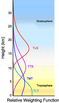
RSS Figure 2. Vertical relative weighting functions for each of the channels discussed on this website. The vertical weighting function describes the relative contribution that microwave radiation emitted by a layer in the atmosphere makes to the total intensity measured above the atmosphere by the satellite.
It is important to understand that the weighting functions are determined by the physics of radiative heat transfer through the atmosphere. They aren’t chosen for their shape. Rather the frequencies are chosen that give the most useful WFs. This graph from RSS shows these WFs. 4 channels labelled TLT (Lower Troposphere), TMT (Mid Troposphere), TTS (Upper Troposphere/Lower Stratosphere) and TLS (Lower Stratosphere).
Notice how the weighting functions stretch across a range of altitudes. TMT & TTS get significant parts of their signal from the lower stratosphere, its boundary being at about 10-12 km. In contrast TLS gets almost all of its signal from the Stratosphere with only around 5% from the Troposphere. The channel labelled TLT is the one used by Eschenbach in his graph of satellite data, both the RSS & UAH analyses of that channel.
What is not clear from the graph above is that these 4 ‘channels’ are actually produced from the data from only 3 sensors. TLS, TTS & TMT are directly calculated from one sensor each - MSU's number 2, 3 & 4 on the older satellites. TLT on the other hand, the one used by Eschenbach, is a ‘synthetic’ channel. It uses additional processing of the data from the TMT readings to try and isolate a signal mainly from the lower troposphere. This was first done by Spencer & Christy at UAH in 1982. In 2005 RSS added a similar synthetic channel. So, channels TLT and TMT come from the same sensor.
But isolating the lower Troposphere was only part of the reason it was created. Look at those sections of the TMT and TTS WFs that stretch up into the lower Stratosphere, and remember that the lower Stratosphere has cooled, more than the Troposphere has warmed. So the TMT & TTS channels have a cooling bias because part of the signal measured by their sensor comes from the cooling lower Stratosphere. So, as far as being measurements of Tropospheric temperature is concerned, it is a physical certainty that TMT & TTS are underestimating the correct values. This is why the TLT synthetic channel was created, to remove this cool bias. But this only applies to the lower Troposphere. We do not have data for the upper Troposphere that doesn't have a cool bias.
So armed with this understanding, what do we see from their analyses. RSS are calculating a trend for TLT of 0.142 C /decade from a TMT trend of 0.087 C /decade. For UAH it is 0.14 and 0.05 respectively. So the processing to extract TLT from TMT is adding a significant amount to the trend. This is the data Eschenbach has based his graph on, although he is only using the land component of the data.
But as we said earlier, three other groups also look at the data. And they report significantly higher values than this.
Fu et al 2004, 2005
In 2004/2005 Qiang Fu, Celeste Johanson et al published an alternative method for removing the Stratospheric bias from the MSU2 (TMT, T2) signal. Since the MSU4 (TLS, T4) signal is predominantly Stratospheric in origin they removed a proportion of the T4 signal from the T2 signal to remove the Stratospheric bias to T2. In order to determine how much to remove, they used radiosonde data to establish a vertical temperature profile for the atmosphere. Then they determine by a least squares regression technique the appropriate weight to give to T2 & T4. Their results are shown below. This calculation was performed in 2004 using data up to 2001. Many of the differences between the RSS & UAH methods had not been resolved at that point. Note particularly how much the RSS and UAH values change between the first and second graph when the Fu method is applied. And the RSS/UAH values here are their TMT values, not TLT.


Their weighting function has a broader weighting over the entire Troposphere than the TLT products (dashed line) and peaks at a higher altitude so is likely to be more representative of the overall Troposphere. NOAA maintains a comparison temperature record for UAH, RSS & the Fu et al adjustments to them here.
Vinnikov & Grody
In 2005 Vinnikov & Grody et al (V&G) published another analysis of MSU data trends. Based on their previous work, it used a quite different, frequency & statistically based method to determine the underlying trends for the MSU measurements. They also consider additional issues related to calibration errors. Instead of assuming that there is a linear calibration error associated with the hot target calibration, they allow for this calibration error varying over the satellites orbit due to external factors. They show that they can calculate this effect based just on latitude/longitude variation of the reading without needing to look at any time dependency.
In their earlier work they had put a figure on trends of 0.22 to 0.26°C/decade. In this work they are estimating 0.20°C/decade. The following graphs show measured Surface, and their calculated TMT trends vs. latitude, and the same values calculated by climate models. The key discrepancies are at the poles with the modelled Northern Surface temps being much higher than measured Northern Surface temps, but modelled and measured Northern Troposphere values agreeing well. Surface temperature products don’t cover the Northern polar region or extrapolate from lower latitude measurements. Southern polar values also disagree but this is commonly ascribed to the effects of the Ozone hole which climate models do not include yet. There is significant agreement at mid and tropical latitudes.


So both these teams have used different approaches to looking at either the calibration and error issues or producing an alternative to the TLT product. But they don’t actually produce a regular time series product because they don’t have the ongoing funding to do so. Just analyses of methods.
Zou et al (Star)
In 2010 Zou et al at NOAA published a new analysis method to produce low level MSU data for TMT. This deals with removing many of the other calibration and inter-satellite correlation issues that UAH & RSS must also tackle but by a very different approach. Their method uses Synchronous Nadir Overpasses – points in time where two satellites are able to observe the same point below. This happens mainly at the Poles. Using this they are able to evaluate most of the onboard & inter-satellite calibration issues since the satellites are receiving the same signal from below at the same time. This method has a lot to recommend it since you can compare apples with apples when comparing two satellites. And this significantly improves how quickly you can establish a basis for comparison between satellites without needing long periods of operation in parallel before you can ‘stitch’ their data together – an issue that plagued the UAH/RSS analyses.
And they are producing on-going temperature series for a range of sensors. The main outstanding area that their analysis does not address is the Stratospheric cooling bias. They are not really trying to do this, instead trying to produce an equivalent to the TMT data series. Their results are shown below. The data from their analysis can be obtained here.

Monthly anomaly time series and trends for the global mean TMT, TUT (their name for TTS) and TLS – the bottom 3 series. The other trends shown are for higher in the Stratosphere.
The key trend we are interested in is the bottom one: TMT of 0.131°C/decade. In contrast to RSS of 0.087 and UAH of 0.05°/decade, this is significantly higher. The Zou group have plans to produce a TLT product from their TMT data although they have not stated whether the methodology used will be the same as the RSS/UAH method.
So what trend would Zou produce if the TLT calculations were added as well? We can’t know for certain yet, but they must be higher than UAH or RSS simply because their starting point from the TMT trend is so much higher. For a definitive answer we will need to wait for their analysis. But we can possibly make a ballpark estimate.
If we simply take the difference between the TMT and TLT values for RSS & UAH as being indicative of how much the TLT processing adds to the underlying TMT trend, and add them to the Zou teams TMT trend we might get some idea:
RSS Values: 0.131 + 0.142 - 0.087 = 0.186
UAH Values: 0.131 + 0.14 - 0.05 = 0.221
Lower Tropospheric warming of the order of 0.2°C/decade. Putting us into the range suggested by Fu and V&G.
So what can we conclude about the Satellites?
Two teams using essentially the same or similar methods are producing trends of around 0.14°C/decade for TLT. Three other teams using three different methods are producing significantly higher values, suggesting 0.18 to 0.22°C/decade. Can we be certain which is correct? No.
But Eschenbach’s assertion that: ‘It’s possible they’re both wrong (UAH/RSS), but that doesn’t seem likely’ doesn’t sound quite so unlikely at all does it?
And if he is wrong, if the higher values from the other three groups are closer to reality, then the satellite records do agree well with expectations and the surface record, then there is essentially no discrepancy to explain. And the proposition that UHI, Station issues etc are either not significant or are well accounted for in the Surface temperature products looks fairly robust. It looks likely that the 'its station issues, its UHI' argument is on its last legs. That one method is right and three other methods are all wrong.
Perhaps the odds that Eschenbach is correct are 1 in 4 – against!
Eschenbach also seems to think that the expectation from theory is that the air in the Troposphere over the land should show greater warming seems to be a confusion of 2 different ideas. Greater warming is expected at the surface on land compared to the oceans since the oceans can transport heat away from the surface down to the depths. Also greater warming at the land and ocean surface in higher latitudes than at the equator is expected since major processes within the climate system transport heat from the equator to higher latitudes.
This is not to be confused with the so-called Tropospheric Hot-Spot. This is driven by quite different involving evaporation from the oceans and is expected to produce greater warming higher in the Troposphere, partiicularly in the Tropics.
So just for interest, lets go back and look at the diagrams from both Fu et al and Vinnikov & Grody. They both show greater warming in the tropics in the Troposphere. As expected, greater warming in the troposphere compared to the surface.
Now lets take a look at 2 MSU channels we have ignored so far – TTS (or TUT for Zou) and TLS. The Upper Troposphere and the Lower Stratosphere. These are both real, MSU based channels, not a derived channel such as TLT. What do they show as trends? We will look at RSS & Zou since UAH don’t process TTS.
TTS TLS
RSS 0.001 -0.303
Zou 0.044 -0.326
TTS shows almost no trend at all while the next layer up, TLS shows substantial cooling. So is the upper Troposphere not warming at all? Go back and look at the weighting functions from RSS. TLS has most of its signal coming from the lower Stratosphere, with negligible signal coming from the Troposphere, maybe 5%. So this must be real cooling in the Stratosphere. But TTS has around 40% of its signal coming from the lower Stratosphere! And it is showing negligible trend. So… if 40% of its signal is coming from a layer showing strong cooling, doesn’t that mean that … the signal for the other 60% must be coming from a region showing strong warming?
Lets do a rough calculation using RSS and Zou to estimate an upper Troposphere temperature trend (Tut)
For RSS we have:
(0.4 * -0.303) + (0.6 * Tut) = 0.001
So:
Tut = (0.001 -(0.4 * -0.303)) / 0.6 = 0.20°C/decade.
And for Zou we have:
(0.4 * -0.326) + (0.6 * Tut) = 0.044
So:
Tut = (0.044 -(0.4 * -0.326)) / 0.6 = 0.29°C/decade.
Could that possibly be the Upper Tropospheric Hot-Spot?
Surely Eschenbach didn’t miss this as well?


[DB] "The whole atmosphere has contracted because of the drop in the solar wind."
Citation, please. Or is this yet another assertion without evidence from you?
[DB] "If you know the reason I am all ears to learn."
Read the links you were given; questions, if any, may be placed there.
[DB] Perhaps you should look into what the thermosphere is...and isn't. Like it's not the stratosphere, for one. You are being off-topic. Cease.
[DB] Try here.
I am having trouble understanding how the MSU works. Let me begin with what I think I do know, and let’s see if that’s OK.
The microwave radiometer measures radiance (intensity) of O2 which depends on the ambient temperature at which the molecule finds itself. Normally selection rules say a homonuclear diatomic molecule (like N2) with no electric dipole is transparent to microwave. OTOH, O2 is paramagnetic so the radiation can couple to the molecule’s magnetic dipole, hence leading to absorption and emission. The radiometer has several channels which detect microwave intensity with a voltage response that is digitized and stored.
Each channel has a voltage vs. atmospheric pressure curve that maximizes at a specific pressure and so specific altitude which is different for each channel. Your article is calling these the relative weighting function.
Here’s the question. What is different about what each channel is measuring, and how do that parameter and the voltage allow specification of the temperature and pressure? I assume each channel is somehow tuned to a different frequency by a few wavenumbers, but I’m not a spectroscopist and haven’t been able to deduce the answer. I haven’t been able to find it on the web either – everything stops short of that kind of detail.
To clarify what I don't know a little further, I am aware of pressure broadening. But even if each channel were measuring line shapes (peak widths), how would you be able to separate different band widths at a given frequency? Perhaps part of the answer is that different rotational transitions might have very different intensities as a function of pressure, but wouldn't they as a function of temperature at the same time? How does all of this get resolved?
tcflood @24/25, the following is the microwave absorption spectrum of oxygen at different altitudes:
The absorption spectrum is a a function of absorptivity, which equal emissivity, so the above graph also tells you the relative strength of emission of O2 if all levels were at a constant temperature.
If you have an instrument on a satellite examining the emissions at 69 Ghz, you would know that it came almost entirely from the lower 3 km of the atmosphere. You know this because the lower 3 km will emit at that frequency, but the levels above that will neither absorb nor emit at that frequency (or at least, not significantly). In contrast, if you sampled at 60.5 GHz, you would know that the radiation comes mostly from 20 Km or above. That would be because O2 at those levels emitt microwaves, but also because they strongly absorb microwaves, thus filtering out the lower levels. By carefull selection of frequency, you can thus choose among a range of emission weights with altitude, which will be governed by the radiative transfer properties at that altitude as modulated by pressure.
If you have a spare $130, this book will give you all the information you desire (I suspect). Unfortunately, I could not find the original proposal for the MSU or AMSU instruments by google search. Should you be able to do so, they undoubtedly be able to give you far more detailed information.
Additional to the above, Chris Colose (I think) once posted a very interesting blog showing satellite images at different frequencies showing clearly how different altitudes became successively revealed. Very interesting inrelation to tcflood's question. I have tried to find it since with no success. If anybody could direct me to it, or the original data he used, I would greatly appreciate it.
Tom Curtis,
Thank you for taking the time to give this detailed answer. It's a big help.