


 Arguments


Challenges in Constraining Climate Sensitivity: Should IPCC AR5’s Lower Bound Be Revised Upward?
Posted on 11 June 2014 by John Fasullo
Equilibrium climate sensitivity (ECS) refers to the global surface temperature change anticipated as a result of doubling atmospheric carbon dioxide concentrations. As it is tied directly to the net climate feedback, ECS is a useful aggregate measure of some aspects of forced climate change. While it is not a fully holistic metric for understanding a broad range of climate change impacts (e.g. it doesn’t address the details of transient changes or changes in other aspects of the climate system such as the hydrologic cycle), ECS exists as a central focus of attention in characterizing the potential magnitude of anthropogenic climate change.
Because ECS is not precisely known it is typically quantified by a “likely range”. Multiple approaches exist for estimating the range, though important differences exist between the ranges provided by different techniques. In IPCC AR4, the likely range was estimated at 2-4.5C. In IPCC AR5, a decision was made to reduce the lower bound of this estimated range (1.5-4.5C), in light of several studies using the surface instrumental record and claiming a lower likely range. Since the submission deadline for inclusion in AR5 (July 2012), a number of important updates to the literature have occurred, including an improved evaluation of
- The contrasting influence of different forcing types on transient changes (aka forcing efficacy);
- The phenomenology of the recent hiatus in global surface warming; and
- The sensitivity of some of the instrumental studies to data used and base assumptions.
Given this progress, it seems reasonable to revisit the decision to reduce the lower bound and ask whether the reduction remains warranted. In short, it is argued here that although IPCC’s conservative and inclusive nature may have justified such a reduction at the time of the report, the evidence accumulated in recent years argues increasingly against such a change.
The Challenge
As outlined above there are multiple approaches for estimating Earth’s equilibrium climate sensitivity (ECS) and transient climate response (TCR). All attempts to quantify climate feedbacks, changes in the climate system that either enhance (positive feedbacks) or diminish (negative feedbacks) the change in the amount of energy entering the climate system (the planetary imbalance) as a result of some imposed forcing (e.g. increased atmospheric concentrations of carbon dioxide). To varying extents, the approaches all face common challenges, including uncertainty in observations and the need to disentangle the response of the system to carbon dioxide from the convoluting influences of internal variability and responses to other forcing, such as due to changes in aerosols, solar intensity, and the concentration of other trace gases. It is known that sensitivity estimates derived from both the instrumental and paleo records entail considerable uncertainty arising from such effects (1, 2).
For some approaches, uncertainty in observations is also a primary impediment. Efforts to estimate climate sensitivity from paleoclimate records are a good example. While benefiting from the large climate signals that can occur over millennia, these approaches face the additional challenge of a proxy record that contains major uncertainty (2). Nevertheless, the paleo record provides a vital perspective for evaluating the slowest climate feedbacks. General circulation models (GCMs) offer a uniquely physical approach for estimating ECS and TCR and readily allow for controlled experimentation, yet their representations of key processes is often lacking (also for example the interaction of aerosols with clouds) and some processes, particularly those acting on low frequency timescales or for which observations are generally unavailable, contain additional uncertainty.
Climatological constraint approaches attempt to relate the spread in these uncertainties across GCMs for some simulated field to a key physical feedback or basic model sensitivity. This approach has led to the developing subject of ‘emergent constraints’ (3,4). Challenges for the approach include the difficulty of establishing statistical confidence in identified relationships, due to a lack of independence across GCMs, and the need to firmly establish a physical basis for why a climatological constraint should act as an indicator of future change. The degree of these challenges may relate to how strongly a given field is tied to surface temperature, as useful insight has been gained for some fields (e.g. snow cover and water vapor; 3,5) but not others (clouds; 6).
The relevance of perturbation studies to climate change are limited by the degree to which they can serve as analogues to climate change, the certainty with which their forcing can be known, and the potentially complex and poorly understood interactions between that forcing and nature (e.g. clouds). So-called combined approaches incorporate two or more of the above methods in an attempt to leverage the strengths of each, but in doing so are also susceptible to their weaknesses. Broadening the discussion to address TCR increases the range of relevant processes to include those governing the rate of heat uptake by various reservoirs, particularly the ocean.
To some extent, the distinctions between ECS estimation methods are artificial. All GCMs have used the instrumental record to select model parameter values that produce plausible climates, and similarly all observational constraints require some implicit 'model' of the climate, even if this is simply an energy balance approach. Ultimately further progress in estimating both ECS and TCR may best be made by a combined consideration of the individual approaches and the adoption of a physically-based perspective rooted in narrowing uncertainty in the individual feedbacks that govern sensitivity across a broad range of timescales.
The Need For Physical Understanding
Irrespective of their complexity, all approaches are faced with the challenges of attribution and uncertainty estimation, for which the validity of observations, underlying model, and base assumptions are key issues. It therefore is inappropriate to place high confidence in any single approach. Given this, and the fact that they do not each lead to the same estimated range of sensitivity, undermines efforts to provide a single best estimate. A complicating factor is that definitions of ECS can vary somewhat within the context of each approach, with estimates of ECS being based on a rather limited set of feedbacks as traditionally defined in slab-ocean GCM experiments (so-called fast-physics feedbacks including those in clouds, water vapor, and temperature), an additional level of complexity in the context of fully coupled GCMs and the instrumental record (including changes in the upper ocean, cryosphere, and vegetation), and the influence of very low frequency processes on paleoclimate timescales (involving ice sheets, deep ocean). A focus on specific feedbacks, rather than on ranges for sensitivity, promotes an apples-to-apples comparison across these perspectives.
A challenge to the feedbacks-centric approach however is that existing multi-model GCM archives contain output that only allows for limited exploration of feedbacks on a process level. Computation of key diagnostics (e.g. atmospheric moisture and energy budgets) is not possible given the limited availability of the high frequency data required, and many aspects of model physics remain undocumented. There is also a need to include experiments that isolate individual feedbacks. It is anticipated that with additional improvements in these archives and strategic experimental designs, many of these issues will be addressed in coming years (7).
Simple Models - When Are They Simplistic?
Simple models rooted in statistics can be powerful tools for interpreting complex systems, a potential that relates to understanding both GCMs and the instrumental record. Ideally, if the appropriate statistical “priors” can be found for the free parameters in the models and if the underlying model is adequate, there is the potential for significant insight. In practice however, the approaches can be severely limited by the assumptions on which they’re based, the absence of a unique “correct” prior, and the sensitivity of their methods to uncertainties in observations and forcing (8, 9).
Simple models are also problematic in that they are of limited use for hypothesis developing and testing. They do not resolve individual feedbacks and thus how to incorporate them in the approach for future progress mentioned above remains unclear. This is not to say however that they offer no potential for hypothesis building. In fact, one hypothesis that has been suggested based on simple models is that the climate record of the past 15 years or so argues for a reduction in the lower bound of our estimated range of ECS, due to the reduced rate at which the surface has warmed and the negative feedbacks it might be viewed as suggesting. Indeed, this hypothesis was found to be sufficiently compelling that IPCC AR5 lowered its lower bound estimate on the likely range for ECS (10). But in retrospect, was this change warranted.
The “Hiatus”: Evidence For Lower Sensitivity?
In the past decade or so there has been a slowdown in the rate of global surface warming. This so-called “hiatus” has been manifested with both seasonal and spatial structure, with greatest surface cooling occurring in the tropical eastern Pacific Ocean in boreal winter and little cooling apparent over land or at high latitudes (9). The apparent slowdown of global surface warming has led some to conclude that evidence for lower climate sensitivity is “piling up” (11). Some have even argued that global warming has stopped.
It is true that, under the assumption of all things being equal, simple models have provided a consistent message regarding the need to lower the likely estimated ranges of sensitivity in order to achieve a best fit to the observational record (12,13). However, per the discussion above, a more physical approach is also essential in order to test this hypothesis and evaluate whether or not the circumstances surrounding the hiatus are indeed suggestive of “all things being equal”. In essence, the physical assumptions underlying this interpretation merit further scrutiny.
If the argument is to be made that recent variability warrants lowering ECS estimates, then clearly a central tenet of that argument is that the planetary imbalance has been mitigated by feedbacks. To reasonably assert that global warming has stopped, the planetary imbalance should be shown to be zero. Such assertions are readily testable across a broad range of independent climate observations and, in fact, a growing body of work has aimed to do just this.
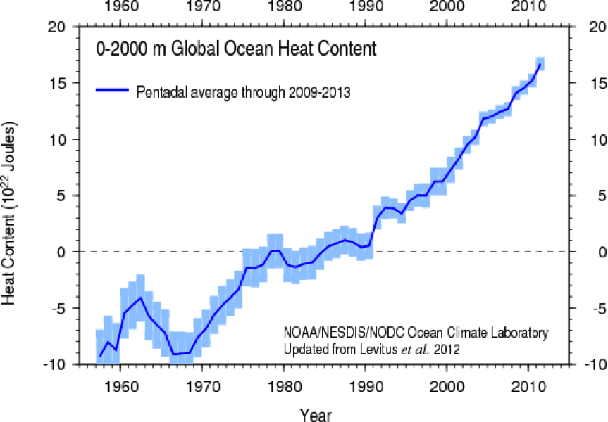
Fig. 1: Global ocean heat content from the surface through a) 700 m and b) 2000m with error estimates (bars) based on data from the World Ocean Database (14).
The picture emerging from this work is that surface temperature during the hiatus has not been driven primarily by a reduction in the planetary imbalance due to negative feedbacks but rather by the vertical redistribution of where in the ocean the imbalance is stored. Specifically, the increase in storage in deeper ocean layers has led to a relative reduction in the rate of warming of the upper ocean. When this vertical structure is averaged out, for example by considering the total ocean heat content (OHC) from the surface to 2000m (Fig. 1) the data show remarkable constancy in the rate of warming from the 1990s through 2000s. They also show a dramatic shift in how that warming has occurred as a function of ocean depth between decades, with the uppermost layers warming little in recent years in conjunction with rapid warming at depth.
The general lack of strong decadal shifts in total OHC have recently been corroborated by estimates of global thermometric sea level rise from satellite altimetry, which show remarkable persistence in the rate of thermometric expansion since 1993 (15). Further, efforts to deduce variability in the planetary imbalance from the satellite record of top of atmosphere radiative fluxes also find little change between the 1990s and 2000s (Richard Allan, personal communication). The consistent picture that emerges from these various lines of evidence is that any assumption of “all things being equal” with respect to internal variability during the hiatus is invalid and little evidence exists for a role played by reductions in the planetary imbalance due to climate feedbacks. In the context of this exceptionally persistent planetary imbalance, studies suggesting a role for reductions in net forcing as driving the hiatus (16) only heighten the challenge for hypotheses that the hiatus is evidence for a strong negative feedback.
Is such behavior surprising? Not really. As early as 2011, a study demonstrated that the NCAR CCSM4 reproduced periods analogous to the current hiatus, with such periods accompanying changes in the vertical redistribution of heat driven by winds at low latitudes (17). Subsequent work has shown that similar behavior is evident across a wide range of GCMs and recent observations have only reinforced the likelihood that the current hiatus is consistent with such simulated periods. The main question that persists relates mainly to the broader context for the hiatus, given the uncertainties surrounding internal variability, and just how unusual such an event may be.
Nature As An Ensemble Member, Not An Ensemble Mean
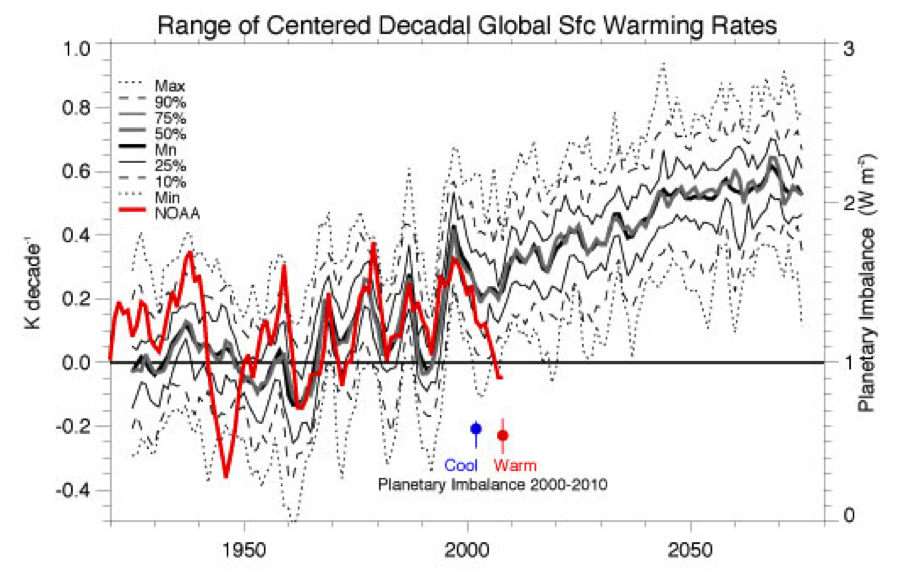
Fig. 2: The range of decadal trends in global mean surface temperature from the CESM1-CAM5 Large Ensemble Community Project (LE, black and grey lines, 18) along with an observed estimate based on the NOAA-NCDC Merged Land and Ocean Surface Temperature dataset. Also shown are the mean (circle) and range (lines) of simulated planetary imbalance (right axis) from 2000 through 2010 for the 10 members of the LE with greatest cooling (blue) and warming (red)
The NCAR CESM1-CAM5 Large Ensemble Community Project provides a unique framework for understanding the role of internal variability in obscuring forced changes. It currently consists of 28 ensemble members in simulations of the historical record (1920-2005) and future projections (2006-2080) based on RCP8.5 forcing.
At 4.1 C, the ECS of the CESM1-CAM5 is higher than for most GCMs. Nonetheless, decadal trends from the model track quite closely with those derived from NOAA-NCDC observations (red line), with the model mean decadal trend (thick black line) skirting above and below observed trends about evenly since 1920. In several instances, decadal trends in observations have been at or beyond the LE ensemble range including intervals of exceptional observed warming (1945, 1960, 1980) and cooling (1948, 2009). The extent to which these frequent departures from the LE reflect errors in observations, insufficient ensemble size, or biases in model internal variability remains unknown. Nonetheless, there is no clear evidence of the model sensitivity being systematically biased high. Also noteworthy is the fact that the LE suggests that due to forcing, as indicated by the ensemble mean, certain decades including the 2000s are predisposed to a reduced rate of surface warming.
The LE also allows for the evaluation of subsets of ensemble members, such as in Fig 2, where the planetary imbalances for the 10 ensemble members with the greatest global surface warming (red) and cooling (blue) trends from 2000-2010 are compared. It is found that no significant difference exists between the two distributions and the mean imbalance for the cooling members is actually greater than for the warming members. Thus the finding of a relatively unchanged planetary imbalance during the recent hiatus period is entirely consistent with analogous periods in LE simulations. While the LE does suggest that recent trends have been exceptional, this is also suggested by the instrumental record itself, which includes exceptional El Niño (1997-98) and La Niña events (2010-2012) at the bounds of the recent hiatus.
A Path Forward
It is likely that a combined effort that makes use of various approaches for constraining sensitivity, with an emphasis on evaluating individual climate feedbacks with targeted observations, provides a viable path forward for reducing uncertainty. Process studies focusing on feedback related fields are also essential and recent efforts have shown consistently that low sensitivity models generally perform poorly and therefore should be viewed as less credible (4, 19, 20). Testing models with paleoclimate archives, where uncertainties in proxy data and forcings are adequately small, is also likely to be essential.
Often lost in the conversation of estimating climate sensitivity is the need for well-understood, well-calibrated, global-scale observations of the energy and water cycles and related analysis systems such as reanalyses to provide a global holistic perspective on climate variability and change. As the hiatus illustrates, such observations can be an invaluable tool for hypothesis testing. Lastly, there is a need to move beyond global mean surface temperature as the main metric for quantifying climate change (21). Improved estimates of ocean heat content have been made possible though data from ARGO drift buoys and improved ocean reanalysis methods. Similar advances are being made across a range of climate indices (e.g. sea level, terrestrial storage) and are likely to be fundamental in providing improved metrics of climate variability and change, evaluating models, and narrowing remaining uncertainties.
References
- Schwartz, S. E. (2012). Determination of Earth’s transient and equilibrium climate sensitivities from observations over the twentieth century: strong dependence on assumed forcing. Surveys in geophysics, 33(3-4), 745-777.
- PALAEOSENS Project Members. (2012). Making sense of palaeoclimate sensitivity. Nature, 491(7426), 683-691.
- Hall, A., & Qu, X. (2006). Using the current seasonal cycle to constrain snow albedo feedback in future climate change. Geophysical Research Letters, 33(3).
- Fasullo, J. T., & Trenberth, K. E. (2012). A less cloudy future: The role of subtropical subsidence in climate sensitivity. science, 338(6108), 792-794.
- Soden, B. J., Wetherald, R. T., Stenchikov, G. L., & Robock, A. (2002). Global cooling after the eruption of Mount Pinatubo: A test of climate feedback by water vapor. Science, 296(5568), 727-730.
- Dessler, A. E. (2010). A determination of the cloud feedback from climate variations over the past decade. Science, 330(6010), 1523-1527.
- Meehl, G. A. (2013, December). Update on the formulation of CMIP6. In AGU Fall Meeting Abstracts (Vol. 1, p. 05).
- Trenberth, K. E., & Fasullo, J. T. (2013). An apparent hiatus in global warming?. Earth's Future.
- Shindell, D. T. (2014). Inhomogeneous forcing and transient climate sensitivity. Nature Climate Change.
- Collins, M., R. Knutti, J. Arblaster, J.-L. Dufresne, T. Fichefet, P. Friedlingstein, X. Gao, W.J. Gutowski, T. Johns, G. Krinner, M. Shongwe, C. Tebaldi, A.J. Weaver and M. Wehner, 2013: Long-term Climate Change: Projections, Com- mitments and Irreversibility. In: Climate Change 2013: The Physical Science Basis. Contribution of Working Group I to the Fifth Assessment Report of the Intergovernmental Panel on Climate Change [Stocker, T.F., D. Qin, G.-K. Plattner, M. Tignor, S.K. Allen, J. Boschung, A. Nauels, Y. Xia, V. Bex and P.M. Midgley (eds.)]. Cambridge University Press, Cambridge, United Kingdom and New York, NY, USA.
- Lewis, N. and M. Crok, 2014: A Sensitive Matter, A Report from the Global Warming Policy Foundation, 67 pp.
- Lewis, N. (2013). An Objective Bayesian Improved Approach for Applying Optimal Fingerprint Techniques to Estimate Climate Sensitivity*. Journal of Climate, 26(19).
- Otto, A., Otto, F. E., Boucher, O., Church, J., Hegerl, G., Forster, P. M., ... & Allen, M. R. (2013). Energy budget constraints on climate response. Nature Geoscience.
- Levitus, S., et al. (2012), World ocean heat content and thermosteric sea level change (0–2000 m), 1955–2010, Geophys. Res. Lett., 39, L10603, doi:10.1029/ 2012GL051106.
- Cazenave, A., Dieng, H. B., Meyssignac, B., von Schuckmann, K., Decharme, B., & Berthier, E. (2014). The rate of sea-level rise. Nature Climate Change.
- Schmidt, G. A., Shindell, D. T., & Tsigaridis, K. (2014). Reconciling warming trends. Nature Geoscience, 7(3), 158-160.
- Meehl, G. A., Arblaster, J. M., Fasullo, J. T., Hu, A., & Trenberth, K. E. (2011). Model-based evidence of deep-ocean heat uptake during surface-temperature hiatus periods. Nature Climate Change, 1(7), 360-364.
- Kay, J. E., Deser, C., Phillips, A., Mai, A., Hannay, C., Strand, G., Arblaster, J., Bates, S., Danabasoglu, G., Edwards, J., Holland, M. Kushner, P., Lamarque, J.-F., Lawrence, D., Lindsay, K., Middleton, A., Munoz, E., Neale, R., Oleson, K., Polvani, L., and M. Vertenstein (submitted), The Community Earth System Model (CESM) Large Ensemble Project: A Community Resource for Studying Climate Change in the Presence of Internal Climate Variability, Bulletin of the American Meteorological Society, submitted April 17, Available here: http://cires.colorado.edu/science/groups/kay/Publications/papers/BAMS-D-13-00255_submit.pdf
- Huber, M., Mahlstein, I., Wild, M., Fasullo, J., & Knutti, R. (2011). Constraints on Climate Sensitivity from Radiation Patterns in Climate Models. Journal of Climate, 24(4).
- Sherwood, S. C., Bony, S., & Dufresne, J. L. (2014). Spread in model climate sensitivity traced to atmospheric convective mixing. Nature, 505(7481), 37-42.
- Palmer, M. D. (2012). Climate and Earth’s Energy Flows. Surveys in Geophysics, 33(3-4), 351-357.
Biosketch
Dr. John Fasullo is a project scientist at the National Center for Atmospheric Research in Boulder, CO. He received his B.Sc. degree in Engineering and Applied Physics from Cornell University (1990) and his M.S. (1995) and Ph.D. (1997) degrees from the University of Colorado.
Dr. Fasullo studies processes involved in climate variability and change using both observations and models with a focus on the global energy and water cycles. He has published over 50 peer-reviewed papers dealing with aspects of this work, aimed primarily at understanding variability in clouds, the tropical monsoons, and the global water and energy cycles. His work has centered on identifying strengths and weakness across observations and models, and has emphasized the benefits of holistic evaluation of the climate system with multiple datasets, theoretical constraints, and novel techniques. Dr. Fasullo is a member of various committees and science teams, and participated in the IPCC AR4 report that contributed to the award of the Nobel Peace Prize to IPCC in 2007
This post was modified from John Fasullo's contribution to Climate Dialogue


"Nature As An Ensemble Member, Not An Ensemble Mean"
If this kind if thing were more widely known and understood, it might take some of the punch out of those "the models didn't predict the Pause!" posts that always swamp the comment threads of any news article about climate change.
Of course, it also helps to understand the difference between a model projection and a climate/weather FORECAST. That's a slightly broader issue, into which the data/ensemble difference can figure neatly.
Frankly I think the general public needs a simple primer on climate modeling, and why you can't just eyeball the typical ensemble mean graph and extract useful information without knowing how these things work. But this primer would have to be a mass-media, mainstream kind of thing that also reaches the audience demographics who need it most. We can't just trust to climate blogs and Youtube presentations to get the info where it needs to go, because self-selection is so very prevalent. Good luck getting Murdoch-owned networks to run such a segment.
Though the discussion needs to move beyond global average surface temperature as the main metric I would prefer to clarify that a global average surface temperature trend based on following average surface temperatures of longer time periods (like a rolling 30 year average) can still be meaningful. A longer time period can reasonably average in the many signficant but randomly fluctuating factors that can affect the global average surface temperature. The 30 year average in the GISTemp data has continued to rise through the past 15 years at a rate of over 0.15 degrees per decade. However, a longer time average could lead the delayers to claim te need to wait 30 more years before deciding if anthing conclusive has been proven. That would not be helpful.
SKS has presented other effective ways of showing the changes by including reasonable adjustments of global average surface temperature for the major variable influences.
The greatest benefit from the continued pursuit of even better way of integrating all the factors will be the improved ability to forecast things like expected regional weather to improve crop performance by better matching planting with the expected regional weather during the growing season, or the improved forecasting of the potential for significant regional weather related emergencies.
The more humanity is able to understand the way our amazing planet functions the easier it will be to develop a sustainable better future for all.
I wonder if the relationship between the estimates of climate sensitivity and the apparent warming slowdown is really there.
The "missing" warming is in the order of 0.1°C for a decade. The man-made warming itself is in the order of 1°C over a century. Thus we are talking about a deviation in the order of one to a few percent.
I would personally not expect that small deviation to influence the estimates of the climate sensitivity that much. Aren't the recent estimates of climate sensitivity lower for other reasons? Or is there some nonlinearity in these estimation methods that I am overlooking?
VictorVenema @3, using HadCRUT4 and calculating the temperature difference of the hiatus as the difference after 15 years between the Jan 1983 to Dec 2012 and the Jan 1998 to Dec 2012 trends, I calculate the temperature difference to be 0.18 C. I use HadCRUT4 because it is the most commonly used of the well known climate indices (even though there are good reasons to think GISS, and now BEST, are better). As a result, it is the temperature index most likely to be used in climate sensitivity studies.
Further, warming from 1910 is about 1 C, but warming from the preindustrial era (and certainly from 1850) is about 0.8 C. The difference is because of a low temperature due to a sequence of large volcanoes in the preceding decades (effectively starting with Krakatoa), and a solar minimum in 1910 as strong, or stronger than that we are currently experiencing. Combining the difference in the values, the "hiatus" would make a difference of 22.7% in a climate sensitivity estimate which was a simple function of temperature and forcing. It would reduce a climate sensitivity estimate from 3 C to 2.3 C per doubling of CO2; or from 2 C to 1.5 C. That is, it is sufficient to account for the reduction on climate sensitivity estimates in the IPCC AR5.
Never-the-less, there are other factors involved. One is lower estimates of the temperature difference between the pre-industrial and the LGM, which has resulted in a number of lower paleoclimate estimates of climate sensitivity. Another is variations of technique such as Nic Lewis's use of a "non-informative prior" which turns out to be an assumption of low climate sensitivity built into the Bayesian methodology (and which is justified only by subjective preference IMO).
Further factors (particularly relevant to Otto et al 2013) include the adjustment of estimated forcings to reflect lower values of aerosol radiative forcing from AR5 (which drops the estimate from 2.4 to 2.0 C per doubling), and the assumption that radiative forcing per doubling of CO2 is 3.44 W/m^2 rather than the more commonly accepted 3.7 W/m^2, without which assumption their estimate would be 2.2 C per doubling. The later assumption is based on Forster et al (2013), who estimate an average adjusted forcing for the CMIP5 models of 3.44 W/m^2. "Adjusted forcing" is a different concept to "radiative forcing", and allows for some rapid tropospheric feedbacks. It is not clear to me that using adjusted forcing rather than radiative forcing in their climate sensitivity estimate is not a mistake.
Finally, some of the perception of a lower climate sensitivity comes from treating all estimates as being equal. They are not. Otto et al, for example state that their estimate is for a "lower bound" of climate sensitivity as it does not allow "... delayed ocean warming at high latitudes can mask the impact of local positive feedbacks". That is, Otto et al {with the probable exception of Nic Lewis ;)} expect climate sensitivity to be greater than their estimate (ignoring error margins), a fact that is frequently ignored.
Tom, you are right, the computation uses the temperature difference and not the energy increase. Does it really just use the temperature difference at the end of the time series? A method that would use the full temperature signal might be less sensitive to natural variability.
Victor @5, I assume by "the computation", you are referring to that in Otto et al. In that case, their preferred value is that derived from the difference between the 1860-1879 to the 2000-2009 intervals. Using HadCRUT4 the trend over 2000-2009 is 0.087 C/decade. The interval is bracketed by the end of the 1999/2000 La nina at the start, and the 2008 La nina, and is either ENSO neutral (NINO 3.4) or has a negative ENSO trend (SOI). For comparison, the BEST trend is 0.116 C/decade over the same interval.
Recalculating the climate sensitivity (ECR) and transient climate response (TCR) using BEST data rather than HadCRUT4, but otherwise using Otto et al's data and methods, I find the following temperature differentials for the various periods used by Otto et al:
That in turns results in the following ECS and TCR estimates, for HadCRUT4:
And for BEST:
From these figures I would find it difficult to argue the slight plateau in temperature increase. One obvious factor is that the difference in ECS or TCR calculated for different periods is entirely a function of differences in temperature. That temperature differential was greatest in the 2000s. Had the temperature differential in the 2000s been at the average value, the ECS calculated would have been 1.2% higher, a difference reasonably attributed to the "hiatus". Further, the RCP 4.5 forcings from CMIP 5 used in the method over estimate forcings in the last 2-4 years of the 2000s, so that there use would underestimate climate sensitivity. This is an indirect consequence of the "hiatus" in that lowered temperaures in those years are partly a consequence of the reduced forcings.
All in all, the temperature difference due to the hiatus may account for a 2% understatement of ECS, suggesting your insight was more perceptive than I allowed.