


 Arguments


Milankovitch Cycles
Posted on 22 July 2011 by Chris Colose
This post is intended to serve as a supplement to SteveBrown’s series on the Last Interglacial, beginning here.
Changes in the Earth's orbit brought about by astronomical variations have a strong impact on Earth’s climate. They serve as the pacemaker for the glacial-interglacial cycles over the Quaternary (roughly the last two and a half million years of Earth's history), and provide a strong framework for understanding the evolution of the climate even over the Holocene (the last 10,000 years, beginiing near the termination of the last glacial period). Milankovitch cycles are insufficient to explain the full range of Quaternary climate change, which also requires greenhouse gas and albedo variations, but they are a primary forcing that must be accounted for.
Orbital variations are also likely to be a generic feature of other planets, with strong implications for the fate of planetary atmospheres (for example, understanding the potential for habitability on other systems). This post will serve as a guide to what these so-called Milankovitch cycles are, how they work, and highlight some "to-be-done" work that remains.
Milankovitch cycles are classically divided into the precession, the obliquity, and the eccentricity cycles. These cycles modulate the solar insolation (i.e., the total energy the planet receives from the sun at the top of the atmosphere) or its geographic distribution. For example, figure 1 shows the solar insolation change at various latitudes in June over the last one million years.
Figure 1: June (daily averaged) insolation (W/m2) over the last 1,000,000 years (0=1950) at (blue= 90 N), (red = 60N), (green =30N), (purple=Equator), (light blue = 30S), (Orange=60S). Data from Berger A. and Loutre M.F., 1991, Insolation values for the climate of the last 10 million years, Quaternary Sciences Review, Vol. 10 No. 4, pp. 297-317
Each of the relevant Milankovitch cycles are described below:
Eccentricity: Eccentricity is a measure of how circular a curve is, with e=0 describing a circle, and e=1 describing a parabola. The orbital eccentricity therefore characterizes how circular or egg-shaped a planet’s orbit around the sun is (Fig. 2). The timescale of Earth’s eccentricity variation is ~400,000 years with a superimposed 100,000 year cycle. There is also an unimportant 2.1 million year cycle.

Figure 2: Circular and eccentric orbit.
Because of eccentricity, the distance of the Earth at perihelion (point closest to sun) is slightly different than the distance to aphelion (point farthest from sun).
Earth’s eccentricity is very moderate, never exceeding approximately 0.07 (almost a perfect circle). The modern day eccentricity is 0.016, and as a result, the solar insolation that hits Earth varies by ~6.4% over the course of a year. There are some more extreme examples: Pluto’s eccentricity is about 0.25, higher than any other planet in our solar system. HD 20782b, a newly discovered exo-planet almost 120 light years away has an eccentricity on the extreme end of ~0.97 (similar to Halley's Comet). Eccentricity can introduce very large "distance seasons" on a planet, although this also depends on the thermal inertia, which is large enough on a body with oceans (or a dense atmosphere) to moderate the changes between perihelion and aphelion. As we will see, Earth's seasonal variations are primarily deterimined by its axial tilt rather than its eccentricity.
Eccentricity is the only Milankovitch cycle that alters the annual-mean global solar insolation (i.e., the total energy the planet receives from the sun at the top of the atmosphere). For the mathematically inclined, the annually-averaged insolation changes in proportion to 1/(1-e2)0.5, so the solar insolation increases with higher eccentricity. This is a very small effect though, amounting to less than 0.2% change in solar insolation, equivalent to a radiative forcing of ~0.45 W/m2 (assuming present-day albedo). This is much less than the total anthropogenic forcing over the 20th century. However, eccentircity does modulate the precessional cycle, as we shall see.
Obliquity: Obliquity describes how tilted a planet’s axis is (Fig. 3 shows the obliquity of eight planets, plus Pluto which is labeled as a planet). The tilt of the Earth is ultimately what allows for the existence of seasons, since the Northern Hemisphere is pointed toward the sun in the boreal summer, and away from the sun in the boreal winter. The tilt of Earth’s axis (in other words, the angle between the spin–axis and a line perpendicular to the orbital plane) varies between about 22 to 25° (currently 23.5°) over a period of nearly 41,000 years, driving changes in the distribution of sunlight between the equator and high latitudes (with more tilt implying more sunlight at high latitudes, and less at lower latitudes; therefore more oblique orbits favor deglaciation on Earth).
Uranus is at the extreme end with a tilt of ~98 degrees; this would induce a very different structure of solar heating (where at certain times the North or South pole would be receiving most of the sunlight, and allow for a large migration of the solar “hotspot” over the course of one Uranian year); this should drive a different atmospheric circulation than on Earth. For highly oblique planets outside our solar system that have a surface, continents at the Polar Regions would be alternatively cooked and frozen, while the tropical latitudes would have two summers and two winters. At large obliquities (greater than about 54 degrees), the poles receive more annual-mean insolation than the planetary equator (Ward, 1974), and thus the annual-mean energy transport by the circulation would be equatorward.
Figure 3: Obliquity of the Planets, and the direction of spin (note that Venus rotates clockwise, in a retrograde fashion). Taken from www.solarviews.com. Click image to Enlarge
Precession: Precession does not describe how tilted the Earth’s axis is, but rather the direction of its axis. This changes what star is the “North Star” over time (today it is Polaris, but near the end of the last deglaciation it was Vega), and as described below, governs the timing of the seasons. This is illustrated in Figure 4 (a and b) below.
Figure 4: a. Schematic showing the influence of axial precession b. How precession changes the timing of the seasons (4b taken from Ruddiman: Earth's climate Past and Present)
There are two key precession effects: axial precession (see an animation here), in which the torque of the other planets exerted on the Earth's equatorial bulge forces the rotational axis to “wobble” like a spinning top; there is also an elliptical precession, in which the ellipse of the Earth itself rotates about one focus. This means that the elliptical shape of Earth's orbit rotates with the long and short axes of the ellipse rotating slowly in space. This moves the positions of aphelion and perihelion.

Figure 5: Change in the Earth's orbital plane. Even if the spin axis always pointed in the same direction (for example, on a perfectly spherical planet) it it would make a different angle with its orbital plane as the plane moved around
Precession also means that the solstices and equinoxes have changed positions, both with respect to the eccentric orbit, and with respect to the positions of perihelion and aphelion. Today, the positions of the solstices and aphelion/perihelion line up closely (Fig. 6), and the Northern Hemispheric summer occurs when the Earth is further from the sun, but this is not always the case.
The summer and winter solstices mark the longest and shortest days of the year, and we see the sun moving back and forth throughout the year between the Tropic of Cancer (23.5 N) and Capricorn (23.5 S), which is a reuslt of the revolution around the sun with a 23.5 degree tilt. Note also that the 90-23.5=66.5 degree mark defines the Arctic and Antarctic circles. At the shortest winter day (winter solstice), no sunlight reaches latitudes higher than this. The equinoxes mark the point where the length of day equals the length of night.
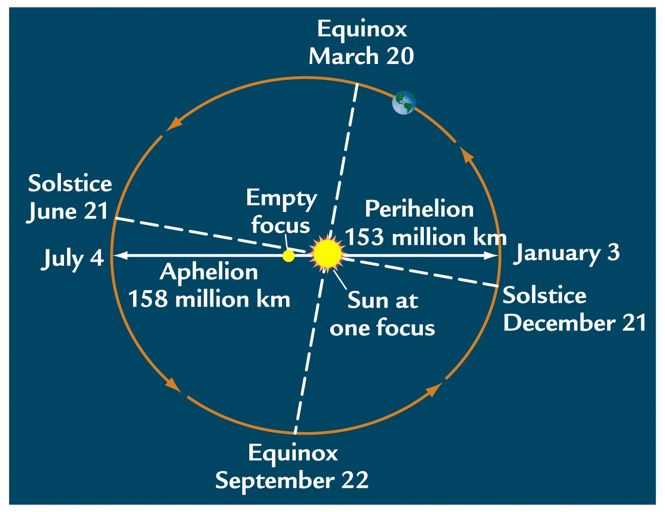
Figure 6: Positions of the Equinoxes, Solstices, Perihelion, and Aphelion. From Ruddimans Earths Climate: Past and Future
Today, the Northern Hemisphere winter occurs near Perihelion, and NH summer occurs when the Earth is farthest from the sun. At present, the Southern Hemisphere has a tendency toward hotter summers , and with a more moderate seasonal cycle in the North, although that simple idea is complicated by differences in land distribution and thermal inertia between hemispheres. However, about 13,000 years ago, the Northern Hemisphere summer would occur when the Earth is closest to the sun, and NH winter when it is furthest from the sun (Figure 4). This would enhance the strength of the seasonal cycle.
Precession varies on timescales of 19,000 and 23,000 years, and is thus important even over historical times. The precessional cycle is the key player behind the Holocene Climate Optimum, a time between ~7,000 and 5,000 years ago of particularly warm Northern Hemispheric extratropical summers, and colder tropical and extratropical winters.
It is important to note that under the precessional cycle, the change in solar radiation striking the Earth is opposite in each hemisphere, unlike the case of obliquity where a higher tilt will mean more intense radiation at both poles as the planet revolves around the sun (although, obviously at the local summer summer for both poles, and thus at different points in the orbit). Furthermore, eccentricity modulates the effect of precession. For zero eccentricity, the precession angle is irrelevant.
What Causes Milankovitch Cycles?
The changes in eccentricity of Earth’s orbit are due to alterations in the gravitational tugs induced by other planets. Jupiter has a very moderate eccentricity, but if it were larger, it would drive larger changes in Earth’s eccentricity. It therefore seems likely that exotic cases of highly eccentric orbits may be prominent in other solar systems, where various gaseous planets are known to exhibit large orbital fluctuations.
Obliquity and precession variations arise due to the torque exerted by gravity (i.e., a force that acts perpendicular to he spin axis of the top) which ultimately comes from the pull of the Sun and Moon on Earth’s equatorial bulge. Precession also varies due to the tilting of the Earth’s orbital plane, as shown above.
The periodicity of Milankovitch cycles is therefore subject to change over geologic time, as the length of day of Earth changes, and the moon becomes further separated from Earth. A shorter Earth-Moon distance would cause the precessional movement to have been larger and the precession and obliquity cycles would have been shorter, as would have occurred in geologically distant paleoclimates. For example, in the Upper Carboniferous (~300 million years ago), the ~41,000 yr obliquity cycle would have taken about 33,000 years (see e.g., here)
Milankovitch Cycles Beyond Earth
Milankovitch cycles are not unique to Earth, nor are the solar system’s orbital characteristics fixed in time. Even our own solar system may be unstable on timescales comparable to its age. In the inner Solar system, the planets' eccentricities exhibit chaos on billion-year timescales (Fig. 7). The lighter planets (Mercury and Mars) have the potential for large variations and in fact, it has been calculated that Mercury has ~1% chance of colliding with Venus or the Sun (or being ejected from the solar system) within the next five billion years (Laskar, 1994, Laskar & Gastineau, 2009).

Figure 7: Numerical Integration describing orbital paramters (10 Byr backward, note this is older than the age of these planets, and 15 Byr forwards). The larger planets behave more regularly. Based on J. Laskar, A&A 287, L9 (1994)
Mars has an obliquity that can vary chaotically between ~0-60°, which has severe implications for its climate evolution. Milankovitch cycles on Mars can actually play a role in redistributing ice on a global scale. In particular, it is thought that deposits of large amounts of water ice recently found in certain areas of the mid-latitudes of Mars (e.g., Holt et al., 2008) must have formed at a time when the climate was conducive to glaciation at middle latitudes, as there is no precipitation in these regions today. This probably requires a higher obliquity, a greater amount of sunlight at the poles, driving sublimation and vapor transport equatorward, where it can then be deposited at lower latitudes (Forget et al 2006). Earth can actually attribute its relatively mild variations in tilt to the stabilizing influence of the moon( Laskar and Robutel, 1993). It would also be possible to have higher obliquity variations if Jupiter were closer to Earth, even with a moon.
Figure 8, below, shows the relatively recent obliquity variations on Mars.

Figure 8: Recent obliquity variation on Mars (-20 Myr to 10 Myr). See Laskar et al (2004)
We don't need to think inside just this solar system though. The influence of exotic spin states or eccentricities is a rather hot topic in the planetary climate community right now (e.g., Spiegel et al., 2010), as new plants beyond our solar system continue to be discovered. Some open questions for example involve the ability to swing in and out of a Snowball planet (or a runaway greenhouse) at highly eccentric orbits. Can planets that undergo large variations in the axial tilt remain habitable? Can planets in binary (two-star) systems be stable? Some of these issues have been explored briefly, but with over 500 planets now discovered outside our solar system and many more expected to come, there's a good amount of work that needs to be done here. Earth, today, is stable in both its modern configuration or in a cold "snowball" configuration (i.e., if Earth were magically ice-covered, it would stay there, even keeping the solar constant and CO2 the same, due to the ice-albedo and water vapor feedback) (Figure 9).
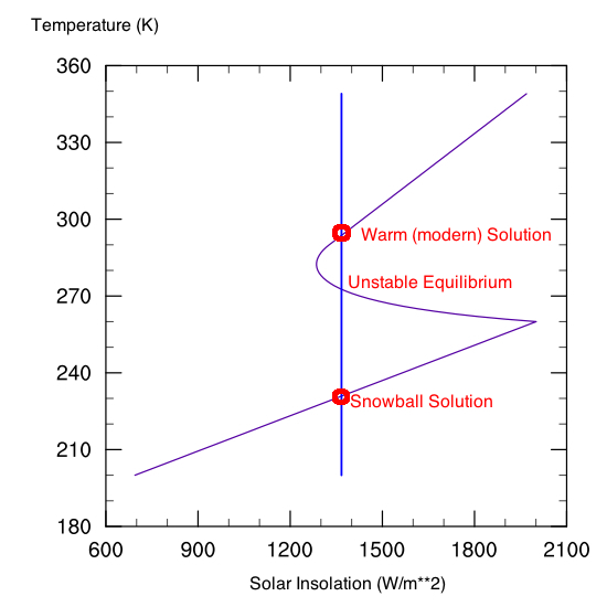
Fig. 9: Bifurcation diagram of Temperature (purple curve) vs. Solar Insolation (blue curve). Because of the ice-albedo feedback, the equilibrium is stable at several points.
Figure 9 cuts into the heart of various planetary climate "extreme" problems. For a relatively circular orbit, the problem of determining where Earth falls into and out of a Snowball is challenging. What happens though if you make the planet slowly rotating? What if the eccentricity is very high, so it the planet swings in and out of the "habitable zone" over the course of one planetary year? Milankovich cycles have the potential to make this issue a lot more interesting, although it is not a solved problem.
Some Final Words
There are still a number of unresolved questions that remain in the astronomical theory of climate change, even during the more familiar Quaternary timeframe. For instance, while we know changes in the orbit pace ice ages, the precise way the three Milankovitch variations conspire to regulate the timing of glacial-interglacial cycles is not well known.
For example, about 800,000 years ago a shift of the dominant periodicity from a 41,000 yr to 100,000 yr signal in glacial oscillations occurred (called the Mid-Pleistocene Transition, see e.g., Clark et al., 2006), and while a lot of ideas exist for why this should be the case, there's no bulletproof answer to this. Explaining the 100,000 yr recurrence period of ice ages is difficult because although the 100,000 yr cycle dominates the ice-volume record, it is small in the insolation spectrum. Therefore, there's still a lot to be done here.
It seems that the Earth listens to the Northern Hemisphere when deciding to have an ice age. If the North and South are alternatively near and far from the Sun during summer, why has glaciation been globally synchronous? What connections are there between Northern insolation and Antarctic climate at the obliquity and precession timescales? What are the competitive roles between a further distance from the sun during summer and a longer summer, following Kepler's law? These quesrions are still not resolved (for a flavor of the discussion, see Huybers, 2009...see also Kawamura et al 2007; Huybers and Denton, 2008; Cheng et al 2009; Denton et al 2010 ). This problem also involves work at the interface of carbon cycle and ice sheet dynamics, processes that are in their infancy in terms of modeling.
Acknowledgments: I'd like to thank fellow SkS contributor "jg" for terrific work in piecing together various visuals used in this post.
Recommended Reading: I also recommend Tamino's multi-part series on Milankovitch cycles (the rest of the posts are linked at the bottom). Involves some math, but a good read.


[DB] Fixed original text.
[DB] The fallacy you fall into is the expectation that hemispherical glaciation is symmetrical, which it is not. Consider the hemispherical distribution of land vs water to gain a sense of the size of the mismatch (and the subsequent relative changes in albedo between glaciation and interglacial).
So your "fact" is completely NOT one.
Dan. I also looked at the Wikipedia entry and wondered about its veracity. Remember. ANYONE can edit wikipedia.
[PS] You are responding to a commentator from 6 years ago. While anyone can edit Wikipedia, the entry contain an excellent set of external links to reliable sources. A google search will find many more.
I know it's an old thread. Huyber and Denton point out that when the NH is intense, the SH summer is longer, and that longer radiation is relatively more effective on the radiative balance when it is colder. Thus the second effect acts at the SH and ties this in to the effects on the NH.
Myself, I have never been able to find a completely satisfactory explanation of the 19 23 41 95 125 413 Kyr cycles, alternatively listed as 21 26 41 96 100 105 108 400, probably varying with orientation to either the eliptical orbit or to the azimuth, etc., but for me incomprehensible.
[PS] Edited for clarity at posters request
stonefly:
Precession means that the orbit maintains the same eccentricity (eilliptical vs. circular), and the earth maintains the same tilt, but the timing during the year of closest/furthest parts of the orbits changes. RIght now, earth comes closest to the sun in January (NH winter, SH summer), and is furtherest away in July. (NH summer, SH winter).
If the opposite were true, - the earth and sun were closest in July, and furthest away in January - we would expect NH summers to be a bit warmer, NH winters to be a bit cooler, SH summers to be a bit cooler, and SH winters to be a bit warmer. So the NH would see greater seasonality, and the SH would see less.
The diagramns above show the same orbit/earth-sun reletaionship and change the labels for Dec/Mar/Jun/Sep. This may be a little hard to follow. Look at the single diagram in the upper left of figure 4, I reproduce it here:
Look a tthe left half only, and think "what would happen if the sun were offset to the right of centre, instead of the left of centre?"
The diagrams in the article keep a different fixed reference, so in the right half the sun and orbit are in the same position but the earth is titled differently. The other diagrams in the change where in the diagram the months are labelled. This is correct in terms of the fixed background positions of the stars, but makes it harder to see that from another viewpoint it is just a matter of which end of the ellipse the sun is located at.
Does that help?
Yes, thank you, Bob.
Then I will assume that the reason precession does not treat the northern and southern hemisphere equally is because of distance.
The sun's rays strike the planet at the same degrees north latitude at perihelion as they strike at south latitude at aphelion, six months later. So it's not the angle of the sun's rays that is affected by precession, it's the distance.
Is that correct?
I see also that at aphelion it is ocean rather than land mass receiving insolation.
stonefly:
I've been AFK, but yes, it's the earth-sun distance variation that causes the seasonal changes. Inverse square law and all that. Combine that with the geographical (land/ocean) difference between southern and northern hemispheres, and you get variations in climate.
As glaciation is strongly a northern hemisphere phenomenon, the glaical periods tend to be linked to periods of low summer NH insolation.
Stonefly @ 42, it might help to consider the effect (or lack of it) of precession when eccentricity is zero, ie if the orbit was perfectly circular (which Earth's orbit never is, but it gets fairly close!). With that orbital geometry, the Earth would be equally close to the sun, and travelling at the same speed, at every point in its orbit. So there would be no differential effect on the hemispheres from the way the planet was oriented during the orbit - eg the NH would not be particularly tilted away from the sun during aphelion, because there would be no real aphelion - it would be the same distance all round the orbit. This is the reason why the eccentricity cycle modulates the precessional cycle; as eccentricity varies, so the impact of the precessional cycles vary. Hope this helps.
Ok a quick question. I am seeing throughout the comments that people are correlating milankovitch's theory with albedo and ocean current to "explain" how solar insolation and ocean co2 can add to the temperature effects of the milankovitch theory. The question that I have is; Is there a way that the extra structures that man have put on the land mass in the northern hemisphere and the factor that we move so much snow to expose the ground to make travel easier possibly changing the albedo effect on solar insolation and combining with our increased co2 output to amplify our current global warming?
Map,
Human constructions like roads and buildings affect the temperature in cities a fair amount. That is called the urban heat island effect. Because cities are relatively small the effect on the Earth's average temperature is small.
To expand your question, land use changes like converting forrest into farmland also affect albeido. Because farms are so large this does have a significant effect on global temperature.
When you make statements like:
" I have decided to abandon the discussion and not educate myself in this area as the "smart people" in the room haven't the ability to portray their thoughts to someone smarter than themselves that just isn't studied in the area he is questioning." my emphasis
You look like you only want to insult people. If you are not informed on the subject we are discussing is is improper to say you are the smartest person in the room.
Michael sweet that quote that you copied from a different page was at someone who was being very judgemental in his responses which is what lead me to that conclusion, which is why I thanked you for your intellectual response before I abandoned my communication with him.
But to continue on your response to my question (which I appreciate). Has land use changes like deforestation for farm ground been compared with the current amplification of global warming to see how big of an affect it is along side with co2?
The change in albedo from human constructions etc. is is under "Land use" in the breakdown forcings.
Source:
This is discussed (with references to the source data) in Chapter 8, section 8.3.5. If you havent already read the the IPCC report, then you should so before leaping in here.
[JH] For future reference, if Map posts comments containing undocumented assertions, please do not respond to them. They will be summarily deleted.]
Michael sweet that quote that you copied from a different page was at someone who was being very judgemental in his responses which is what lead me to that conclusion, which is why I thanked you for your intellectual response before I abandoned my communication with him.
But to continue on your response to my question (which I appreciate). Has land use changes like deforestation for farm ground been compared with the current amplification of global warming to see how big of an affect it is along side with co2?
[DB] Deforestation is about 11% of the overall problem. The human burning of fossil fuels is pretty much the rest.
Scaddenp thank you, that graph show exactly what I was looking for. Interesting that it shows the opposite of what I was comprehending before with the albedo on land mass.