


 Arguments


Science of Climate Change online class starting next week on Coursera
Posted on 17 October 2013 by David Archer
This is a repost (with a few amendments) of a post by David Archer at Real Climate.
Maybe you remember the rollout a few years ago of Open Climate 101, a massive open online class (MOOC) that was served sort of free-range from a computer at the University of Chicago. Now the class has been entirely redone as Global Warming: The Science of Climate Change within the far slicker Coursera platform. Beginning on October 21, the class is free and runs for 8 weeks. The videos have been reshot in a short and punchy (2-10 minute) format, for example here (8:13). These seem like they will be easier to watch than traditional 45-minute lectures from a classroom. It’s based on, and will show you how to play with, all-new on-line computer models, including extensive new browsing systems for global climate records and model results from the new AR5 climate model archive, an ice sheet model you can clobber with slugs of CO2 as it evolves, and more. Come and watch the train wreck join the fun!
Course content
 The class follows the general structure of Open Climate 101, based on the textbook Global Warming: Understanding the Forecast. This is class about science, but it is intended to be understandable by people without a strong science background.
Weeks 1-4 start from the very simplest model for the temperature of a planet, and build a picture of the complexity of the real climate system on Earth, with the greenhouse effect and climate feedbacks.
Weeks 5-6 consider the past and future carbon cycle.
Weeks 7-8 explain where we are and what can be done.
New On-line Climate Stuff
Coursera seems like a powerful medium for teaching any topic. But my class in particular is like no other Coursera class that I’ve heard of, in that it offers a suite of on-line interactive models that you can see here. They are always up and publicly available, so you teachers can throw students at them, no problem.
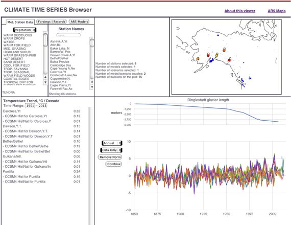
A time-series browser provides access to the GHCNM (NOAA link is currently shut down) global meteorological station monthly mean temperatures (7169 stations), and global glacier length records (472 records). These records can be compared with climate model results from the new AR5 model results, extracted from their grids. There are 12 different models and four scenarios, including Historical, HistoricalNat (natural-only), RCP2.6 (an optimistic ramping-down scenario), and RCP8.5 (less optimistic). This is a very open-ended system; my intent is to allow students to investigate a topic of their own devising, which they will write up and submit to grading by other students, a bit of Coursera wizardry.
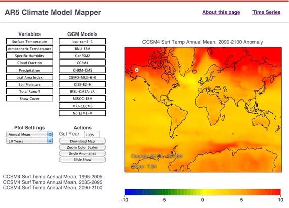
An AR5 output mapper makes colored maps of output from climate models, including 3-D atmospheric temperature, specific humidity, cloud fraction, and 2-D fields of precipitation, soil moisture, runoff, leaf area index, and snow cover. These are monthly mean values from the Historical then RCP8.5 scenarios. The browser buffers the maps so that you can switch between them quickly, or show them in a slide show or movie. This is only a tiny fraction of the AR5 model respository, but it’s still enough data (about 130 GBytes) that serving this to a large MOOC audience is going to be a challenge.
The time-series browser and the map maker are both designed to be easily extended (by me, not by users). The system takes AR5 netcdf files directly as they download from the CMIP archive, and new climate records can be added to the time-series browser as simple csv format. Maybe Skeptical Science readers or students in the class will have suggestions of what to add (I almost hate to ask!).
A new model for comparing the climate impacts of CO2 and CH4, called the Slugulator, lets you release slugs of either greenhouse gas and compare the antics that ensue. A favorite feature of mine is the comparison of the energy yield from fossil fuels, next to the total greenhouse energy trapped over the lifetimes of the gases.
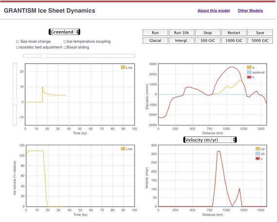
And we have an interactive ice sheet model, you can clobber with slugs of CO2 (or just drag the temperature around) as it’s running. This comes from Frank Pattyn’s Excel-based GRANTISM, recoded as javascript by Martin O’Leary. I added the replay button and the CO2-clobbertron myself, however.
Plus there are retreads of the old favorites like Modtran, with which you can demonstrate the band saturation effect, Geocarb, which shows the long tail of fossil fuel CO2 in the atmosphere, and lots more.


To join in on all the interesting ways of presenting interactive information, I have been adding climate models to my environmental context model server:
http://entroplet.com/context_salt_model/navigate
This particular example demonstrates how natural fluctuations contribute to the temperature pause.
Archer has certainly been improving his online apps, as the Modtran interface has gone through an upgrade. Other good online applications include Climate Explorer, of course the ones here at SkS developed by Kevin, Nick Stokes' Moyhu work, and WoodForTrees.
Hi David,
Thanks for that course. I was a fan of your Modtran model. I'm looking forward to some good in-depth learning of Carbon cycle (i.e. 3 stages of ocean sink as I learned them from Archer 2005) and experimenting with the new models. Perfect content and perfect timing for me.
Thanks again
I have watched David Archers original videos of his lectures based on his book.
I found them very useful in understanding the basics, so I imagine the new course will be just as good with the new materials and additional learning facilities that Coursera enables.
I'm teaching a section on climate change and the censoring of science in my Theater and Justice Class at John College of Criminal Justice: dramatic readings An Enemy of the People, my play Extreme Whether about climate change scientists and deniers, and Euripides The Bacchae. I've gathered some basic readings about climate change, but wonder if you have suggestions. I would also hope to see climate change and global warming integrated more broadly into (what is left of) The Humanities.
I think I see a way to improve the lecture a bit:
The videos (as in the above example tagged: here (8:13) ) which is less than 10 minutes lecture - is a more than 400MB huge *.MOV file.
Maybe the lecture videos should be added into YouTube-format for easy broadcasting without having to download locally?
The underlying Planck distribution for the free website "Modtran Infrared Light in the Atmosphere" is displayed in the user output for a range between 100 wn and 1500 wn. I have accidentally found out that this wavenumber range is not just a graphical convenience. The underlying program does have this somewhat limited wavenumber range.
If one investigates the output of the "Show Raw Model Output" button, two features become evident:
1. The underlying computer program does really have a range limited to 100 wn - 1500 wn.
2. The underlying computer program assumes an earth surface emissivity of 0.98.
I have developed corrections to "Modtran Infrared Light in the Atmosphere" for several fundamental cases. The corrections could be made to a class by verbal instructions and do not require any re-writing of the program.
I submitted an authorship proposal to the "Bulletin of the American Meteorological Society" (BAMS). The suggestion of the Board of Editors of BAMS is the following:
"Your corrections to Modtran sound promising for a wide audience. However, the editors feel that BAMS is not the appropriate venue for vetting and distributing this information. For proper exposure and discussion, they would be more productively disseminated directly within the Modtran user community online." In the spirit of the suggestion of the BAMS editors I post below the first of my corrections.
[JH] Embedded url into free website "Modtran Infrared Light in the Atmosphere".
Correction number one:
Consider the following settings for "Modtran Infrared Light in the Atmosphere" (MILA)
1. All greenhouse gas concentrations set to zero.
2. 1976 U.S. Standard Atmosphere.
3. Looking down from 70 km
4. Temperature offset at minus 33.2 K, giving a grount temperature of 255 K.
The out going long wavelength radiation (OLR) is then given by MILA as 225.075 W/meter squared.
From the "Black Body Calculator" of SpectralCalc, at 255 K, emissivity 0.98, in the 2 wn to 100 wn range the band radiance (SpectralCalc terminology) is 0.554602 W/meter squared steradian. Multiply by the pi available steradians of a Lambertian surface to obtain a flux of :
(a) 2 wn to 100 wn outgoing flux of 1.742 W/meter squared.
By a similar procedure for 1500 wn to 2200 wn one obtains
(b) 1500 wn to 2200 wn flux of 6.3437 W/meter squared
Then for the 0.98 emisivity case the corrected MILR output is 225.075 plus 1.742 plus 6.3437 = corrected flux of watts/meter squared of 233 watts/meter squared. This is what one obtains by using an expanded wave number range from 2 wn to 2200 wn, assuming emissivity of 0.98.
If instead of an emissivity of 0.98 one uses an emissivity of unity then by a similar procedure one obtains a corrected output flux of 1.777 w/meter squared plus 231.144 watts/ meter squared plus 6.473 watts /meter squared equals 239 watts/meter squared. Note that here the output of MILA between 100 wn and 1500 wn is changed from 225.065 watts / meter squared to 231.144 watts per meter squared to correspond to emissivity of one instead of the MILF emissivity of 0.98.
The context of these results is the following: A number of treatments of elementary environmental science, such as written, for instance by Archer or by Wolfson, show that an Earth with no greenhouse effect, but assuming a best estimate of cloud albedo, is in thermal equilibrium with incoming solar radiation if the average Earth surface temperature is quite close to 255 K. This temperature corresponds to an OLR of 239.7 watts/meter squared for thermal IR emissivity of one, by using the Stefan-Boltzmann law. The best value from sophisticated satellite analysis for the top of the atmosphere by Trenberth, Fasullo, and Kiehl, BAMS 90, 2009, 311 - 323 is 239 watts/meter squared. These authors assume an emissivity in the thermal IR for the Earth's surface of 1.0.
I will wait to see if others accessing Skeptical Science and reading this post believe my analysis is correct or not, before posting my next correction which is for the value of the cloud free earth OLR.
In order to proceed further with my corrections to Modtran Infrared Light in the Atmosphere (MILA) I need to include some background material. Here are results for OLR of CO2, only greenhouse gas, U.S.standardatmosphere Modtran. I use SpectralCalc atmospheric paths radiance calculator, looking down. A virtual source is on the Earth's Surface, operating between the 500 wn and 850 wn of the CO2 bending mode. Temp 288.2 K, emissivity 0.98 to match Modtran. In addition to the 500 - 850 wn window the transparent (for CO2, although not water vapor, this will come up later) bands between 100 to 500 and 850 to 1500 wn are included, again to match MILA conditions. The "diffusivity approximation" as described, for instance on the Science of Doom website in part 6 of "The Equations" under the Greenhouse Effect, is used with an effective 54 degrees angle to the vertical to go from upward intensity to OLR with units of w/meter squared. It is not a good match to SpectralCalc to actually use angled paths, for one thing the angled paths in SpectralCalc are "real" paths which are strongly refracted. The "diffusitivity" approximation needs idealized straight line paths. In expressions for the optical thickness the factor q/cos theta always appears, where q is a concentration of the GHG, which in the case of CO2 can be considered constant up to 100 km. Say theta was chosen to be 60 degrees. Since cos 60 degrees is (1/2) the factor q/cos 60 = 2q/cos0.
Therefore one just needs to keep a vertical path and multiply the concentration by 2. In my case I use an effective angle to vertical of 54 degrees and multiply the q by 1.7. Modtran actually integrates over the output angles from 0 to 180 degrees. I calculate for a vertical path with q = 683 ppm for CO2 to compare with Modtran for 400 ppm. Below are the results in the next post.
Altitude in km, OLR in W / M2
Altitude S.Calc 683 ppm Modtran 400 ppm
0 360.2 360.2
1 357.5 357.6
2 353.1 352.9
3 348.5 348.5
4 344.5 344.4
5 340.2 341.0
6 336.4 337.5
7 333.1 334.4
------------------— skipping several entries
18 320.8 324.6
Only major isotopologue of CO2 used in Spec Calc results. Again, 0.98 Earth surface emissivity. Constrained to 100 wn to 1500 wn. For CO2 the windows between 2 wn and 100 wn, and 1500 wn and 2200 wn are transparent. But this is not true for water vapor.
Correction number two
Clear sky OLR measurements from satellites are of considerable interest since the properties of the atmosphere are being studied without the complications of cloud cover. For the "Modtran Infrared Light in the Atmosphere" (MILA) leave all default settings of greenhouse gases in place but choose the U.S. Standard atmosphere with no clouds. The uncorrected clear sky output flux observed by the virtual observer at 70 km is 260.2 W/m2 .
It should be kept in mind in what follows that unlike CO2, which maintains a constant concentration up to ~ 100 km, the water vapor content is concentrated close to the Earth's surface. (This may be seen by clicking the "temperature" button underneath the plot of altitude versus temperature in MILF, and compare CO2 andwater vapor on the drop down menu.)
Using the same SpectralCalc atmospheric path radiance application described in the previous two posts, I set the water vapor scale of the water vapor path to 1.7 instead of the default 1.0. This corresponds to the diffusivity approximation with an effctive angle to verticalof 54 degrees as described in the previous two posts. The radiant emission is calculated for the bands between 2 wn to 100 wn and 1500 wn to 2200 wn, again as described above. These outputs are associated with water vapor since the atmosphere for these wavelength ranges is essentially transparent to CO2 but the water vapor is a strong absorber. For a .98 emissivity, the corrected OLR is 266.7 W/m2 . If the Modtran output is - in addition to adding the pieces between 2 and 100; 1500 to 2200 wn, adjusted to correspond to an emissivity of one for the Earth's surface, the clear sky OLR becomes 272.1 W/m2 . This is compared to the value of the clear sky OLR obtained by Chen, Huang, Loeb, and Wei using the AIRS spectrometer of 273.74 W/m2
Chen, et al "Comparisons of Clear - Sky Outgoing Far IR Flux Inferred from Satellite Observations....." Table Three, Journal of Clima,Vol 30, No 9, May 2017.
curiousd
Just a point of clarification. MODTran is a commercially available medium resolution Radiative Transfer Code. It is developed by the US military, primarily through the Air Faorce laboratory system, although they outsource the actual coding. In contrast the Uni of Chicago is hosting a copy of MODTran and supplying configuration parameters to it for their web interface and then showing results from their run.
So the criticisms you are making are more likely related to the configuration setup by UoC not anything built into the software itself which is a more general purpose tool. The emissivity of 0.98 for example would be their setup parameter, and is actually a reasonable average of the actual emissivities of materials on the Earths surface which tend to range between 0.96 to 0.995. Similarly the wavenumber range will be a choice by UoC, rather than built in.
curiousd
Here is a link, from the UoC site, to a technical summary of MODTran from the company who wrote the code - Spectral Sciences Inc. Note the distribution list to the Air Force. Note on the first page of the introduction, the range of wavenumbers is from 0 to 17,900 cm-1. This upper limit is defined by the range of the data in the HiTran database, not a limit in the code per se.
http://climatemodels.uchicago.edu/modtran/berk.1987.modtran_desc.pdf
Glenn, I don't think I am criticizing the Modtran site at all. It is an excellent teaching tool and my point is that an instructor could use these corrections along with Modtran to better illustrate certain important results. For instance, I suspect most students would never look at the underlying program button, and therefore simply stating someplace on the web site or in classroom hand outs that an emissivity of 0.98 is assumed and there is a cut off issue would improve things.
As a case in point, I myself went down the following dead end regarding the emissivity issue. If one simply takes the MILA OLR looking down from the surface and compares to what is expected from the Stefan Boltzmann law you appear to have an emissivity of 0.92 because of the cut offs at 100 wn and 1500 wn. But at time I was using MILA for my purpose I had no clue about the cut offs and assmed the program must assume an emissivity of 0.92.
If someone is using the MILA program to test whether he/she is correctly using Scwarzchild's equation to obtain, say, the co2 no feedback climate sensitivity---where else can you obtain the OLR versus altitude, even in any textbook?---that person will run into contradictions with such a low assumed emissivity. (This is the subject of my next post here.)
All this would be improved just by warning the user of the wavelength cutoffs and that the assumed emissivity is 0.98 not 0.92 on the output website the user uses. The way I discovered this, after months of work, was to digitize the output of MILA and integrate the case of co2 only at 400 ppm and then test my use of the trapezoid rule for integration. I happened to have used an underlying Planck distibution that went from 5wn to 2000 wn. My answer for the integration was significantly too large. So I changed the range of the integration to 100 wn to 1500 wn and got close to the MILA output.
Then I knew.
curiousd @6-10,
The first question to ask you is - Have your "corrections" been "disseminated directly within the Modtran user community online" ? As you report @6, it is the advice of the BAMS editors that you should do this. It would also be my advice.
The two "corrections" you describe here (if I understand correctly) concern firstly the impact of IR beyond the range 6.67-100μm which you calculate as being significant yet outside the calculations made by the MODTRAN model, and secondly the lack of spherical adjustment for height in that model.
Regarding the first of these, using the on-line calculator at SpectralCalc.com, the value of blackbody radiation beyond 6.67-100μm amounts to 3.6% at 255K. I would assume the creators of MODTRAN were not unaware of that situation when they determined the wavelength limit of the model.
Regarding the second correction, the spherical effect on IR flux over 70km of atmosphere would be about 2%. While this may or may not be of significance to the MODTRAN model, the adjustment you make to the MODTRAN inputs to simulate this effect is surely incorrect. Your adjustment is "multiplying the standard ropospheric water vopor concentration" by 1.7. Concerning your use of Chen et al (2013) to provide a check on your correction, you should note that the value in Chen el al Table 3 is a "near-earth global annual mean" and so not actually comparable with any setting available on the MODTRAN interface. Those settings only provides for certain 'Locality' and weather, settings which greatly impacts the "Upward IR heat flux" . Thus your 260.2w/sqm is calculated from MODTRAN applies only to "1976 U.S. Standard Atmosphere" and "No Cloud or Rain".
I thank M.A. Rodger for his critique; it is exactly what I want.
(1) I can think of no other way to "disseminate the corrections to the Modtran online community directly " than to post such corrections as I have developed on "Skeptical Science" and "Science of Doom".
(2) The corrections I have made use SpectralCalc, a relatively inexpensive and wonderful tool for learning or teaching about atmospheric science. It would go well with Modtran. I can go further and take my violation of the plane - parallel approximation into account.
(3) I am not sure what you mean about the 1.7 factor being the correction I make. The1.7 factor is to expand the underlying wavelength range in the most correct way; to make the most "correct correction" . I cannot (or have not yet taught myself how to do it) actually integrate the intensity over many different angles. Modtran Chicago does this; that is better than my method, which is to use the "diffisivity approximation" approach and multiply by pi whilst at the same time effectively switching from a vertical path to one at 54 degrees. My table in post nine shows that by using a vertical path corresponding to 693 ppm - which has the identical effect as a straight line path at 54 degrees and 400 ppm - I can nearly duplicate the Modtran result for "CO2 only" where the Modtran result is for 400 ppm but they integrate outgoing intensity over all directions. I then carry over the 1.7 so that my "correction is more correct" for the water vapor bands. My correction is to expand the band width to 2 wn through 2200 wn from the original 100 wn to 1500 wn.
With respect to the comparison to Chen, et al: Since I use the U.S. Standard Atmosphere, which is supposed to be a type of world wide average, why is it so unexpected that my result isclose to that of Chen, et al ?
(You get something pretty close to the correct CO2 only climate sensitivity if you use MILA in U.S. standard atmosphere and the 0.98 emissivity; despite the fact that the present best value is by Myhre, who I believe found it improved the result to average over many locations? M.A. Rodgers, is the previous italacized sentence correct ?)
Also, regarding your criticism: Thus your 260.2w/sqm is calculated from MODTRAN applies only to "1976 U.S. Standard Atmosphere" and "No Cloud or Rain".
The idea of a "Clear Sky" OLR measurement is to obtain the OLR with no clouds or rain. Otherwise it would not be a clear sky experiment.
curiousd
The person to contact regarding this would be Professor David Archer at UoC. The Modtran calculator site is part of a set of tools he uses in running on-line courses about climate science.
d-archer@uchicago.edu
Hi Glenn,
But not before what I havedone is thoroughly vetted, as the editors of BAMS suggest. The only way to thoroughly vet this is to continue to post my arguments and have experts at S.S. try to shoot them down. I suspect that the place where the largest effect ofthe correction is would be in estimating the relative contribution of CO2 relative to water vapor on the earth's temperature, since the tails between 2 wn and 100 wn, and 1500 to 2200 wn have extremely strong water vapor absorption but negligible CO2 absorption. I am building up to this.
curiousd @15,
I should confess that my comment @14 was quite a bit more than I had initially intended to say, and I can see I have erred in places (but only in places).
Concerning your "Correction Number One", the value presented by the UoC calculator as 'Upward IR Heat Flux' is calculated over the range 100cm-1 to 1500cm-1 and I think we can say with confidence that such a restricted spectrum will be ignoring 3.6% of 255K blackbody radiation spectrum. Of course, the TOA spectrum is only a very very approximate blackbody spectrum. I did a very quick scaling of this graph which plots TOA flux from 0cm-1 to 2000cm-1 and suggests there is somewhat less than 3.6% unaccounted, perhaps only a further 2% in the 0cm-1 to 2000cm-1 range leaving potentially 0.5% of unaccounted blackbody radiation above 2000cm-1.
It seems I was in error interpreting what your "Correction Number Two" was about. On reflection, your second correction appears to be suggesting that MODTRAN does not correct for the horizontal component of radiative transfer. This I cannot believe. And I fail to grasp the logic of your correction - increasing water vapour by a factor of 1.7 (=1/cos54º, the angle being the average for the integral). If such a correction were to be made, surely it would also require a similar adjustment to all other GHGs.
Chen et al (2013) does indeed concern clear-sky data (specifically 2004 data) and thus is comparable with 'No Clouds or Rain.' Note that Chen et al compares observations with reanalyses which use MODTRAN5 to calculate the TOA spectra flux. The comparisons of flux over the spectrum 0 – 1800 cm-1 are scattered either side of the observation with roughly 1% accuracy. This result suggests that MODTRAN in an apples-v-apples analysis does not need correction. The use of the 0 – 1800 cm-1 spectrum also reduces the blackbody IR beyond the range 100cm-1 to 1500cm-1 to 2.8% and scaling that graph of TOA IR it reduces to 1.4%.
Concerning the use of 1976 US Std Atmosphere. This is a global average for the full annual cycle and with non-liner calculations such an average cannot be as acccurate as the Chen et al analysis. If the impact of using a spectrum 100cm-1 to 1500cm-1 is roughly 2%, a little under half of the descrepancy you set out @10, it may be worth considering if a less crude averaging method can be shown to reduce that remaining 3%.
There may still be other explanations. It is not impossible to believe that the UoC calculator contains simplifications (as yet undiscovered by us) even though it produces some very convincing-looking outputs.
As I said, increasing the water vapor concentration by 1.7 is only because it has precisely the same effect on the radiation emitted as using a 54 degree angled path, even though I am using a vertical path. This is because 1 / cos 54 degrees is 1.7/cos zero degrees. The angle 54 degrees is by some measures, close to the optimum angle to do this.
Here is another way of looking at it. Consider the equation for a "path" such as in equation 4.67 in Pierrehumbert for the strong line limit in the Curtis-Godsen Approximation. There is a factor in the equation for the "path" LS which is q(p)/cos theta. The q(p) refers to the specific mass as a function of pressure. The equivalent width of a Lorenzian line is given by W = 2 x sqrroot (S(Tnought)*gamma (p0))* times LS where LS is the "strong path" (Pierrehumbert top of page 230.) Gamma (p0) is the line width at surface atmospheric pressure. S(Tnought) is the Line Strength analagous to a mass absorption coefficient at the surface of the Earth, where in this approximation one neglects the temperature dependance of the Line Strength. This is all part of an old way to estimate transmittance values without cranking out a line by line result. q(p) is a specific mass which may vary with height ; therefore pressure. Thus, it is a constant for CO2 up to order 100 km; however, water vapor is concentrated near the Earth surface. But no matter; a vertical path (cos zero = 1) ; using 1.7 times q(P)) is mathematically exactly the same as q(P) in the numerator and cos 54 degrees in the denominator. Now that we have SpectralCalc to hand us transmittance values on a platter, it is much easier and quicker to merely multiply the q(P) by 1.7 instead of actually changing to an angled path.
The chief technical person for "SpectralCalc" has told me that the same issue comes up in their radiance programs as in old ways of computing transmittance. Using a 54 degree angled path whilst multiplying the quantity with units of (watts / square meter steradian wave number) by pi is a" quick and dirty approximate way" of converting to diffuse upward flux by averaging over all angles.
The SpectralCalc expert has told me that the SpectralCalc way is to use a "fourth order quadrature" but what I do is a "quick and dirty way to proceed."
Bottom line..what MILA does is to angle integrate all angles and do it correctly. I do not know how to do this, so I use the old recipe for converting intensity to OLR by multiplying by p1 and effectively using a 54 degree straight line path.
(This is sometimes called the "diffusivity approximation" see Science of Doom under greenhouse effect, part 6 the equations , or page 171 in Grant Petty's text book for a drawing of the method. Also see in Liou, p. 127. Liou states that "in general a four point Gaussian quadrature will give accurate results for integration over the zenith angle"..but "for many atmospheric applications it suffices to use (shows equation involving the diffusivity factor.) See Pierrehumbert on page 191 who describes the method at length and even compares the various angles one might use.
Note that 400 ppm x 1.7 is 680 ppm. In my post 9 above you will note that for CO2 if I use a factor of 1.7 to multiply the 400 ppm present day CO2 concentration but do not integrate over angles then I get good agreement with MILA for 400 ppm where they do integrate over angles.
I think we should get this straight before talking about the other issues.
curiousd @19.
It seems we discuss a work by Pierrehumbert. It would be good to be sure we are discussing the same work so a proper reference would be good. The work you reference should be listed here although likely it will be this work you offer up for discussion. (By the way, my initial thought @14 had been solely to provide the links, not to comment on them.)
Hi M A Rodger,
The reference is my well worn copy of "Principles of Planetary Science" ,Raymond T. Pierrehumbert, Cambridge University Press, third 2014 printing, ISBN 978 - 0 - 521 - 86556 - 2 Hardback. Some time ago in a completely different context I was given an URL for a free online copy by someone on SS. Maybe Tom Curtis??? Even then there is a strange thing...almost all of the ONLINE version is the same as the book, but some of the book material has been left out. Maybe I can dig up the URL to the on line version someplace on my computers, but no guarantees.
Hi M A Rodger,
Look at http://cips.berkeley.edu/events/rocky-planets-class09/ClimateVol1.pdf
Unfortunately the thorough discussion of the various angles one might use under different circumstances on page 191 in my text does not appear to be in this. However, page 190 does have the statement after equation 4.69 "For strong lines the equivalent width is...." Note that within the radical is the symbol L sub S for the "strong path". Note that in equation 4.67 the set of terms q(p)/ g cos theta appear together. The q(p) is not a constant as it is for CO2 up to 100 km, but if I multiply by 1.7 the factor 1.7 being constant comes outside the integral. This complication does not come about for the CO2 case since q is constant and comes outside the integral.
I am assuming that SpectralCalc correctly takes care of the integral of q(p)dp between pressures.
BTW..One of the limitations of both MILA and Spectral Calc is that both have no ability for the user to resolve altitude steps less than 1 km. Of course, both MILA and SpectralCalc have a length resolution much less than this in the underlying program. For MILA I think I recall from the button for the underlying program that the length resolution is one centimeter. MILA is free, SpectralCalc is amazingly reasonable and Modtran6, which I have also purchased is expensive! But with Modtran six, one has a resolution in length at least down to a meter, a wavenumber range way more than I would ever need, and it deals with scattering. But although I am quite familiar with SpectralCalc I can now only do rudementary things with Modtran6, just because I have not studied the program very much. It is breaking in a new GUI interface, other wise I never would have purchased this package.
Curiousd @19.
While we have now both sourced Pierrehumbert, are now looking at the same writing, and while you do say “I think we should get this straight before talking about the other issues“, do note my apprehension expressed @18 concerning the use of the 1976 US Std Atmosphere as a global average.
In producing a better global average than the single values fo single the 1976 US Std Atmosphere, the UoC model does provide regional/seasonal alternatives for analysis. I have endeavoured to gain a global average by weighting these regional/seasonal UoC alternatives. Using the surface temperature outputs from the UoC model, the weighting that provided a parity of global average temperature is 50% tropics and 12½% for the 4 remaining latitude/seasons. This is not an unreasonable outcome. It would fit with global coverage 70ºS to 70ºN. (The Chen et al analysis coverage is 80ºS to 80ºN.)
The calculated TOA IR flux from the UoC model when weighted in this manner yield a global average global of 265.9Wm^-2, a significant increase on the 1976 US Std Atm output. If the 1½% to 2% is added to this sum (representing the additional IR in the 0-1800cm^-1 band used by Chen et al but excluded by the UoC model (your 'Correction Number One'), we arrive at a TOA IR flux range of 270-271Wm^-2. These values are now very close to the measured global value used by Chen et al (273.7Wm^-2) and their calculated values (271.7, 274.2, 277.0Wm^-2) . That the UoC calculator comes so close is pretty impressive for a webpage-calculator.
O.K...but think that in correction number one I used the unscreened output of the 1500 to 2200 wn band. I think that this does not represent the actual output if water vapor is included. Also recall that in correction number one the output is for 255 K.
Using the SpectralCalc black body calculator set at 0.98 emissivity one obtains:
The unscreened output is 19.35 watts per meter squared for a temperature of 288.2 K for a band from 1500 wn to 2200 wn.
For a band from 1500 wn to 1850 the unscreened output is 14.752 watts per meter squared.
The band from 2 wn to 100 wn produces an unscreened output of 2.02 watts per meter squared.
(a) Total corrected (unscreened by water vapor) flux is then for 2 wn to 1850 wn
260.2 + 14.752 + 2.02 = 276.9 watts per meter squared.
(b) Total corrected flux (unscreened by water vapor) for 2 wn to 2200 wn band is then
260.2 + 19.35 + 2.02 = 281.57 watts per meter squared.
The second total is too large. If I replace the 260.2 watts per meter squared by your 265.9 watts per meter squared then (a) becomes 282.672 watts per meter squared and (b) becomes 287.27 watts per meter squared and now both (a) and (b) are too large.
The question of adjusting from the 1976 Standard atmosphere is one thing, and I'd want to learn more about this. Looks interesting. What is most clear, in my opinion, is that this correction cannot be carried out without putting the water vapor in there. For another thing one wonders: If the piece from 1850 wn to 2200 wn adds so much flux, how could Chen et al just eave it out?
This is all interesting and I appreciate your input and comments.
There is now a practical Skeptical Science question I have....A long time ago I knew of the way to make graphs and paste them into these comments, but now Ihave totally forgotton. I will ask in the Newbie section probably Tom Curtis to once more educate me on this.
http://IMGUR.com/a/UMUR1
Please highlight, right click,and go to the URL. I could not get the image to load directly. Sorry.
This image has to do with the last correction,"Correction Three" to MILA
Refer to the image you get from post 25 above. For a CO2 only GHG atmosphere these are plots of the in band outgoing radiance, in w/meter sqd steradian, for wave number range 500 wn to 850 wn CO2 bending mode, versus Earth Surface thermal IR emissivity looking down from zero km and from 1 km. I use a 680 ppm CO2 concentration because this is the present day concentration of 400 ppm multiplied by 1/cos 54 degrees, and 1/cos 54 degrees is 1.7 . Therefore a vertical path with 680 ppm has the same optical length as 400 ppm at a 54 degrees angle relative to Nadir. Therefore I can use this application of the "diffusivity approximation" as a decent substitute for actually integrating over all angles when I multiply by pi streadians to obtain out going flux in W/meter squared. This has been discussed previously by myself and M.A. Rodger here. See posts above 9 and 24.
Of interest here is the sign of the difference between the 0 km and 1 km output. This difference is, for the MILA emissivity of 0.98, given in post 9 and is for the OLR where multiplication by pi steradians has been carried out, equal to 360.2 w/meter square minus 357.5 w/meter squared. Then the OLR at 1 km is about 2.7 watts per meter squared less than at zero km.
In the figure for the URL given above, the multiplication by pi steradians has not yet been carried out and for emissivity of 0.98, the surface upward in band radiance exceeds that of the same quantity at 1 km by 43.5764 minus 42.7272 or 0.8492 watts /meter squared steradian. Multiply this quantity by pi steradians to obtain a result which is 0.8492 times pi and rounds off to 2.7 watts per meter squared, in agreement with post 9 above.
However, note in my figure you can see at the URL I refer to above, the value of the one km in band radiance decreases at a rate less than that of the zero km in band radiance as the emissivity is decreased. In fact, for surface emissivities of 0.93 or less the upward in band radiance at 1 km is greater than the upward in band radiance from the surface.
I was surprised at this result, but it has to do with Correction Three since the sign of the difference between OLR surface and OLR 1 km changes sign between emissivity of 0.98 and 0.92.
The "apparent " emissivity of MILA obtained just by looking at the output without knowing the settings of the underlying program or knowing about the 100 wn to1500wn truncation, is not 0.98 but 0.92.
This can lead astray anyone wishing to check if they are using Schwarzchild's equation correctly to compute the CO2 outgoing flux, by usig MILA. And where else can the user find a set of OLR values such a at MILA to test if she/he is doing things correctly?
I will let this post "subilate" a bit before proceeding. The finding that one can have OLR at 1 km greater than at zero km seems surprising, and my only justification so far is that: 1. I use a procedure with SpectralCalc that give good agreemen with MILA and gives an expected CO2 climate sensitivity of ~ 4 watts/meter squared. 2. That applying that procedure to low emissivities of 0.93,0.92,0.91, 0.9, and 0.89, gived me the result that the OLR from 1 km exceeds that from the surface.
I believe that desert aras have such low emissivities.
Of course an emissivity in the thermal IR less than one implies some scattering or reflection, so that likely must be considered. BTW SpectralCalc gives the caveat that they do not deal with scattering in any way; just absorption and emission.
Also, regarding to explaining correction three, the following comparison might be useful.
Modtran Light in the Atm SpectralCalc Modtran6
PRICE free $ $$$$
dist resolution 1 km 1 km < 1 meter
maximum alt up to 70 km error message if TOA
>"1 million point error" exceeded
if too much band width
or altitude. Therefore simulating a 54 degree angled path by multiplying the input concentration can be possible whilst extending path length not so much
curiousd @24,
To recap my postion on your "Correction Number One" which concerns an underestimation by UoC MODTRAN model (aka MILA) of TOA IR flux due to the limits of the wavelength used in the UoC model.
@7 you calculated a potential value of this correction as 9W/sq m, roughly 3.6% of the UoC calculated average global value.
@18 I argue that this value is too high, presenting two reasons for my lower estimate of roughly 2% or 5W/sq m.
@24 you are now calculating the value for this "Correction Number One" as if the extented spectrum (beyond that used in the UoC calculation) has zero GHG acting in it. The value you calculate 14W/sq m is thus a maximum value for "Correction Number One" which would be valid only for a zero or very small GHG effect in the wavelenghts being considered. As the graph I linked @18 shows, there is a large GHG effect in these wavelengths and the large correction you suggest @24 is unjustified.
curiousd @26,
You state that your "Correction Number Two" has been discussed with me up-thread. My position concerning the existence of your "Correction Number Two" remains as stated @18 - "This I cannot believe. And I fail to grasp the logic of your correction." Our discussion has not developed beyond that point (other than sorting out some references).
Concerning your "Correction Number Three," I fail to see the origins of the "One km" IR Radiance values in the graph linked @25. The "Surface" values are evidently blackbody calculations which are thus much dependent on emissivity. Indicative of the emissivity value (E) is the Peak Spectral Radiance (PSR) which for a blackbody temperature of 288.2K would be:-
E/PSR, 0.92/0.125, 0.94/0.128, 0.96/0.131, 098/0.133, 1.00/0.136.
Examination of the UoC output file for 1976 US Std Atmosphere (288.2K) yields a maximum PSR of 0.133 W/sqm/sr/cm^-1 which indicates Emissivity = 0.98. The Band Radiance from the UoC calculations (43.589 W/sqm/sr for 500-800cm^-1) also suggests Emissivity = 0.98.
It is unclear to me how you are calculating the 1km Band Radiance values. (You give the Emissivity = 0.98 value for 1km as 42.7272 W/sqm/sr which I note is very similar to the UoC value for Band Radiance 490-860cm^-1 42.756.) It is also unclear why this would indicate an Emissivity of 0.92.
Lets deal with correction number one first. Of course I set all GHG equal to zero. Basic texts on environmental physicssuch as the one by David Archer or the one by Wolfson, consider the case where the cloud albedo is kept, but the GHG effect is "turned off". The equilibrium temperature of such an earth, given an emissivity of one, is 239.7 degrees K. For Modtran Chicago, U.S. Standard atmosphere, and 255 degrees K, no GHG, the OLR is 225.07 W/msqd. If I add my corrections to Modtran for 0.98 emissivity I get not 225.07 W/meter sqd but 233 watts per meter sqd. There is no curvature of the Earth effect because if I look at the output from Modtran with zero GHG then the OLR is stays essentially constant but shows some small scatter all the way from altitude zero to altitude 70 km.
The tenberth reference is to show that the most modern satellite result is 239 watts/per meter squared at the assumed emissivity of 1.0.
If I pare my correction down to this statement are you good with this?
Correction: The equilibrium temp is close to 255 K in the above, not 239.7 K. I was confusing the temperature with the flux in this sentence. It has been a long night.
Regarding "It is also unclear why this would indicate an Emissivity of 0.92."
Here is how you get the emissivity of 0.92.
(a) You know nothing about the limited wavelengh range.
(b) You wish to compare the OLR output of MILA with your efforts as someone who is trying to learn how to use the Schwarzchild Equation.
(c) You therefore determine what the MILA emissivity is (with no knowlege of the cut offs or of the actual 0.98 emissivity)
(d) You therefore go to the U.S. Standard atmosphere and learn that the upward OLR from Modtran looking down from zero altitude, is 360.472 W/m sqd.
(e) You use the Stefan Boltzmann law with emissivity one and T = 288.2 degrees K. You get 391.164 K.
(f) You divide 360.472 by 391.164. Your answer is 0.92
Here is a general description of my knowledge of Atmospheric Physics and how I got where I am with such projects as trying to make sure I have applications of the Schwarzchild Equation correct. I was a condensed matter experimentalist with perhaps 75 publications in refereed journals. I also taugnt Freshman Physics of the Environment for many years. Upon retiring I decided to try and learn how to really calculate quantities such as the CO2 no feedback climate sensitiviy and therefore:
I bought large numbers of Atmospheric Physics books and tried to teach myself; my home institution has no one working there who knows the first thing about Atmospheric Physics, so this project has been attempted without human input or correction. Many hours a day were spent on this project and now three years have elapsed. My Rosetta Stone has been the text by Grant Hill, and I think now I have a decent general idea for a one dimensional version of these things.
But it is my opinion that even though Atmospheric Science is certainly correct, it is explained rather poorly to scientists not in the field and for one reason above all: There is a dearth of numerically worked examples for the most important things. Symbolic explanations alone are insufficient.
How could there be, for example, no worked numerical example for the solution to the Schwarzchild Equation for an atmosphere with 400 ppm CO2 to give the upward flux as a function of altitude? Regular Physics is not like this. The students start out learning F=Ma and then M = F/A. In a more advanced class the solutions to the one dimensional Schroedinger Eq. is worked out for any number of potential well problems. E&M is replete with boundary problems involving Gauss' Law.
I think that not having a worked example for the solution to Schwarzchild Equation, given the transmittance values one now has worked out for the user by SpectralCal, is like having no worked examples of the work energy theorem or momentum conservation.
My mistaken derivation of an emissivity of 0.92 for MILA was one of many stumbles that I have had to deal with. If there were merely a statement on the user output page of MILA that (1) an emissivity of 0.98 is assumed that would be agood thing. And if the statement were made that (2) the wavenumber band the computer uses is limited 100 wn to 1500 wn which can introduce errors so the user should be cautious would also be a good thing.
Curiousd @29.
The 255k-239.7W/sqm is a standard blackbody calculation for emissivity=1 with the outward IR flux matching the absorbed solar radiation, thus the albedo remains from cloud & surface while GHG=0 because it is a blackbody. In terms of accurate measurement/assessment of the flux, today there is an energy imbalance due to AGW.
The UoC model gives 226.363W/sqm for 255K (and altitude =0) because emissivity=0.98 and the model only considers part of the spectrum, the value 226.363W/sqm being not greatly different from the 266.52W/sqm value calculated for the part-spectrum using SpectralCalc.com. (The difference is insignificant and could result from many understandable approximations.) Note the implications of this @31.
Putting #31 to one side and assuming your “corrections to Modtran for 0.98 emissivity” are not what is meant, but rather the +8W/sqm you argue for @7. (I miscalculated this as 9W/sqm @28) I set out @18 why I consider this +8W/sqm to be too high and that a +4W/sqm would be more appropriate. You present no reason for the +4W/sqm being incorrect.
The impact of altitude on the flux magnitude has been considered up-thread but as my misinterprettion of your “Correction Number Two”. (Note that I did not indicate the sign +/- @14. In truth I had in mind a positive correction but it would actually be a negative correction.) The UoC model set with GHG inputs as zero does demonstrate a change in flux with altitude but it alters by less than the variation of area with altitude (the square of the effective radius). Thus with all GHGs reduced to zero in the UoC model, we should see a 2.2% reduction from surface to 70km. The actual reduction (varies with surface temperature) is roughly 0.5%. This is probably explained by the continued presence of minor GHGs in the UoC model which are not zeroed but remain unchanged with user input. If this is not the case & if there is no alternative explanation, if it does require correction, this would comprise a reduction of some 4W/sqm for 255K surface and a measured IR flux at 70km.
curiousd @31.
What you demonstrate here is that yor correction for emissivity ("Correction Number Three") is duplicating your correction resulting from the limited spectrum under analysis ("Correction Number One"). When you say "(a) You know nothing about the limited wavelengh range" you correct by adjusting the emissivity value ("Correction Number Three"). But we do know about the "the limited wavelengh range" and when we correct for it ("Correction Number One") the flux calculations match blackbody conditions for emissivity=0.98 as the UoC model says it uses.
curiousd @32.
I am pretty hazy about Schwarzschild but I would not expect there to be a significant gravitational effect (?! I am pretty hazy!) when calculating the radiation flux through a planet's atmosphere.
Regarding:
"What you demonstrate here is that yor correction for emissivity ("Correction Number Three") is duplicating your correction resulting from the limited spectrum under analysis ("Correction Number One"). When you say "(a) You know nothing about the limited wavelengh range" you correct by adjusting the emissivity value ("Correction Number Three"). But we do know about the "the limited wavelengh range" and when we correct for it ("Correction Number One") the flux calculations match blackbody conditions for emissivity=0.98 as the UoC model says it uses."
The 0.92 emissivity result is a problem whether or not one obtains better values for the OLR at 250 K by correction one, or an improved clear sky OLR from correction two. It results in a result for the solution to the Schwarzchild Equation (S E) ,assuming no scattering (two stream approximation), that has entirely the wrong OLR for the 1km distance from ground if the emissivity is 0.98. To the point that instead of a 1 km OLR that is slightly less than the surface ORL, as is the case for 0.98 emissivity, at 0.92 the OLR is slightly greater at 1 km than the surface emissivity.
So consider the "serious user" of MILA who:
1. Assumes that 0.92 is the emissivity instead of 0.98 by doing the simple calculation above comparing the MILS emission from the ground and comparing to the Stefan - Boltzmann law.
2. Correctly numerically applies the SE expression for the outgoing stream in the two stream SE, perhaps applying the SE to only the difference between the 800 ppm and 400 ppm cases for CO2 to get the climate sensitivity. He /She is (unknowingly) using a drastically too low surface emissivity.
3. Since the upstream solution is I^(0) t* plus atmospheric contribution , if I^(0) is (0.92/0.98) factor too small relative to what one gets from MILA, since the atmospheric contribution term is independant of the surface, both the 400 ppm and 800 ppm contributions will be too small relative to what one obtains by just running MILA for 400 ppm and then 800 ppm and subtracting, where the dicrepancy is not much at,say, 20 km but really serious at 1 km.
4. The user will therefore conclude that his/her application of SE is incorrect even though it is not. The user is just (unknowingly) using the wrong emissivity.
Grant Petty states, on his page 215 that the I^(0) term is the "....only term whose value cannot be directly computed from knowledge of (symbol for wave length specific linear absorpion coefficient as function of z ) and (symbol for transmittance as function of z) alone (for given wavelength and viewing direction mu). " He then states:
"The expression we supply for I^(0) depends on what we assume about the nature of the surface. But regardless of those assumptions, there are two contributions that must be considered: (1) Emission by the surface itself, and (2) upward reflection of atmospheric radiation incident on the surface."
I am certain that MILA does not take reflection at the surface into account which is fine for an illustration for students, but then the value of the emissivity of the surface strongly influences both the OLR and the value of intensity 400 minus intensity 800 as function of altitude z.
So back to the serious user of MILA...He/She will think the emissivity is 0.92 instead of 0.98 and therefore get something that disagrees strongly with MILA at 1 km even though that serious user has been applying the SE correctly but whilst (unknowingly) using the wrong emissivity.
curiousd @various, it was established in 1997 by Myhre and Stordal that using a single atmospheric profile in LBL and broadband radiative models will introduce inaccuracies to the calculation. That result was confirmed by Freckelton et al (1998). Myhre and Stordal state:
It follows that if you really want to test Modtran for bias, you would need to use (ideally) 2.5o x 2.5o cells based on weekly averages, and take the means. Failing to do so will introduce a bias, which based in Myhre and Stordal, is approximately equal to 50% of the bias you claim to have detected.
The University of Chicago version of Modtran does not permit that, restricting choices of atmospheric profiles to a Tropical zone, two Mid Latitude zones (summer and winter) and two Subarctic zones (summer and winter). Using default values for a clear sky, and with no GHG I found the difference between the OLWR at 70 km for each case, and for a areal and temporally weighted zonal means, and for the US standard atmosphere at default temperatures, and at a temperature adjusted to match OLWR to the average incoming radiation to have a mean bias of 5.35 +/- 3.69%. Tellingly, the least bias (2.33%) was found with the weighted means. The US standard atmosphere with surface temperature set to 254.5 K showed a bias of 4.19%. Given this, the case for any significant bias in the calculation of OLWR over the range of wave numbers covered by the model is unproven. Given the wide range of biases in different scenarios, it is not clear a single correction factor would work in any case.
Further, the idea that Modtran should be adjusted to determine a single OLWR value seems wrongheaded. Modtran is intended to predict observed IR spectrums given a knowledge of surface conditions, and trace gas and temperature profiles. Here is an example of such a prediction (strictly a retrodiction):
Clearly the University of Chicago version of Modtran is capable of reasonable but imperfect predictions of such observed spectrums. Given the limited ability to reproduce actual conditions (ie, site specific surface emissivity, specific temperature profiles, density profiles, etc) we do not expect anything else, in what is simply a teaching tool. Nor is any explicit bias obvious from the example above, with OLWR at specific wave numbers sometimes being over estimated and sometimes under estimated by the model. If you trully wanted to test Modtran 6 for bias (or for error margin), you would need to compare by wavenumber across a large, but representative range of such site specific profiles.
I have not been following the technical discussion above at any depth, but it seems to me that before you get to that discussion, you need to allow for the known constraints on any radiative transfer model, regadless of its accuracy line by line. Further, you would be better directing the technica discussion to the actual use of radiative transfer models rather than their use (and potential misuse) in testing zero dimensional first approximations of the greenhouse effect.
Hi Tom Curtis,
ModtranChicago is designed primarily for aid in teaching basic environmental science, and is an excellent tool for doing so as is.
It is, as far as I know, also the only source available to everyone for free of plots of outgoing OLR values as a function of altitude and GHG composition. Therefore, for someone such as I, who wishes to learn about at least the one dimensional version of atmospheric science on his own with no available guidance, the temptation will be to use the ModtranChicago output; there is no other choice.
But as is, ModtranChicago gives in its output no information, either for the assumed emissivity or about the restricted underlying wave number range of 100 wn to 1500 wn.
That user will deduce an emissivity of 0.92, which I now know, but did not always know, is entirely too low. See the post 31 above.
That user may then be applying the Schwarzchild Equation correctly and still will find very poor agreement with his "Standard" which is the output of ModtranChicago, for the region near 1 km. The user will then go back to the drawing board repeatedly to find his mistake.
curiousd @36:
Anybody using the UChicago version of Modtran will see in the user inteface a button labelled "Show raw model output". If they press that button, a new tab will open showing that output. Scrolling through it, they will see first the details about the atmospheric profile, absorber amounts etc, and will then come to a section labeled "RADIANCE(WATTS/CM2-STER-XXX)", which is then shown for wave numbers from 100 to 1500 cm^-1. At the bottom, the output shows the "INTEGRATED ABSORPTION FROM 100 TO 1500 CM-1". A little below that it informs us that "BOUNDARY EMISSIVITY = 0.980". In short, all the information you claim is not available, for which according to you, there is "no information" in its output, is all available just by pressing a button of mysterious function with the mystical label "raw model output" /sarc.
Beyond the false claim about what was not available in the Modtran output, there is nothing in your comment not dealt with by my comment to which you were responding.
curiousd @32.
I have tracked down this Schwarzchild Equation and, rather than the ones that explains the wobbles of the planet Mercury, it is a rather mundane equation that I didn't appreciate had a name and which is explained here. Frankly, I do not see how it could be used with the UoC MODTRAN model in a way that would lead to a misapprehension that emissivity=0.92. As Tom Curtis points out @37, the emissivity value is set out clearly in the output file which would be required reading for any "serious user."
Concerning the effect of using a single MODTRAN calculation as a global average, further rough calculations suggest to me that the impact of latitude and the annual & diurnal cycles do appear to provide enough additional flux above that single average figure to add 1% to 3% to the total. While these rough weighted calculations remain very sensitive to the assumed weightings, the outcome appears quite clear. Tom Curtis @35 adds weight to this finding. Add in the truncated frequency used in the UoC model analysis and the flux values are become very close to the Chen et al (2013) values.
Of course this does not mean there is no room for other approximations with significant effect on the result within the UoC model, or even errors. But if you wish to establish the potential of your "Correction Number Two" and your "Correction Number Three" you will need to present due reason. So far, that has not been done. And failing to explain your ideas, for instance the derevation of the "One km IR Radiance" values in the graph you presented up-thread (ie this graph), is not winning you any favours.
Note to Tom Curtis comment 37. I had always assumed, say for two years or so, that I could never understand anything that button revealed, as it would have something to do with the program source code. It was only when I determined by integrating one of the outputs by using a digitized result with an underlying width which by accident extended between 5 wn to 2000 wn and got a significantly larger OLR than was given in the MILA output, and then found I was within 2% of the MILA output if the underlying interval was limited to 100 wn to 1500 wn. that I realizedsomething was wrong.
By user output I meant what the user sees in the window that appears when you click on the URL for MILA. Then I looked at that button and found that the actual integration was limited to 100 to 1500 wn and that the emissivity was0.98 The way I found this out, and that indeed the information was revealed by that button, was described earlier in the thread, Tom Curtis, which you might have looked at more carefully before accusing me of a false claim.
Regarding comment 38. Here is how I get the upward intensity as a finction of emissivity and altitude.
For the zero altitude in band intensity I go to the SpectralCalc black body calculator APP and calculate the in band radiance for 288.2 degrees and the emissivity I put in. I use a wave length range of 500 to 850 wn which completerly includes the bending mode band of CO2.
For CO2 the bending mode range is contained within the 500 to 850 wn range. The band from 100 wn to 500 wn is completely transparent if CO2 is the only green house gas, which I also put into SpectralCalc. The same is true for the window between 850 wn and 1500 wn. Therefore, since CO2 is completerly transparent for 100 wn to 500 wn, and 850 wn to 1500 wn I also obtain those intensities using the SpectralCalc Black Body Calculator as described above in this post. The upward intensity for a CO2 only atmosphere, will be the same for all altitudes for those two outer widows, as observed at ground level, and therefore I just add them at higher altitudes to the output I get for the 500 to 850 band.
For the 500 to 850 band I use the "Atmospheric Paths" APP of SpectralCalc. This gives either transmittances or radiance outputs. Here I use the radiance output. The way this works is that there is a virtual source at ground level, for which you can put in a temperature of 288.2 degrees and an emissivity of choice. Again, I choose an atmosphere with only CO2, major isotopologue. A complication is that the U.S. Standard atmosphere is used in the scale factors. Therefore a scale factor of one does not correspond to 400 ppm of CO2, since back in the 70s the CO2concentration was less than this. For 400 ppm you must therefore use a scale factor of 1.212. The U.S. standard atmosphere is default for the SpectralCalc atmospheric path sections.
Here is my only non standard step: I use instead of 400 ppm a concentration of 1.7 times 400 ppm or 680 ppm. This corresponds to a scale factor of 1.212 times 1.7 or 2.06. Why do I do this? I am in effect using the "diffusivity approximation" as described in great length both in Pierrehumbert's text and Grant Petty's text. The idea is that if one does not wish to integrate the output radiance to obtain diffusive flux, one can approximate the result of integrating that radiance by multiplying the in band radiance by pi and simultaneously replacing all paths involved by a straight line path going at angle theta relative to vertical. Here I quote from the pages within Pierrehumbert that are not available in the URL http://cips.berkeley.edu/events/rocky-planets-class09/ClimateVol1.pdf
Quoting from Pierrehumbert p. 191: "...if the radiation field remains approximately isotropic, the decay rate is the same as for unidirectional radiation propagating at an angle theta such that cos theta = 1/2, i.e. 60 degrees..." Then "..the choice of cos theta = 1/2 is by nomeans a unique consequence of the assumption of isotropy....(under certain conditions) cos theta = 2/3 and this would ve an equally valid choice within the limits of the isotropic approximation..."
Petty staes on page 214..."The most commonly used value of (symbol for one over cos theta) is 5/3"
Note that my 1.7 factor is 1.666 or 2.3 rounded off and my angle is 54 degrees, not 60 degrees.
Furthermore in The Physics of Atmospheres by John Houghton third edition he states on pp. 11 - 12 that for Schwarzchild's Equation, to a good approximation the intensity may be replaced by the diffuse upward flux if B(T), [B(T) is the symbol for the black body emission per unit solid angle per unit area of a surface at temperature T] is replaced by pi B and the incremental increase in altitude dz is replaced by 5/3 dz."
At one time I went through the procedure of replacing vertical angle paths by paths at 54 degrees using a spread sheet. But I realized that exactly the same result is obtained by keeping the path vertical and replacing the concentration q by 1.7 q. Mathematically this must be the case since all the expressiont for transmittance in Pierrehumber involve the set of symbols F (q, theta) = q/cos theta. In the bottom of page 229, Pierrehumbert, his equation for the transmittance between pressures p1 and p2 is one minus the equivalent width where the equivalent width of a single Lorentzian line is one over delta (delta is he range of wave number considered)
time 2 times the square root the hitran line strength for a Lorentzian at at the base of the atmosphere times a different "strong line strength LS". The strong line strength contains together the set of symbols F = q/cos theta. This can be expanded to give the Curtis-Godsen approximation. I have tested whether the transmittance values I get from SpectralCalc and transform to angled paths at 60 degrees using a spread sheet are identical to the transmittance of a vertical path with q' = 2q . The agreement is exact!
Say I chose theta to be 60 degrees. Since for a vertical line cos theta is one, and 2q/one equals q/cos 60 degrees what I do is exactly equivalent to the "diffusivity approximation"
Bottom line....what MILA does is actually integrate over all angles. I use this approximation instead. The techical consultant at SpectralCalc tells me that what I am doing is an approximation to doing this a better way, where he would have used a "fouth order quadrature" whatever that is. He also told me that the same thing is true for the radiant atmospheric path APP as for the transmittance paths in Schwarzchild Equation, i.e. by multiplying the path length by 1.7 or by multiplying the concentration by 1.7 I can approximate the best way of going from intensity to diffuse flux which would use a "fourth order quadrature".
It works!! See post 8 above. The Science of Doom describes the method in their section on the "Greenhouse Effect" "The Equations"
You should also know that if you use atmospheric paths that are too long you get an error message in SpectralCalc to the effect that you have exceeded the one million point limit. Also, their are angled paths already available in SpectralCalc but they are real paths which are strongly refracted, and you need idealized paths that go in straight lines to use this approximation.
In the above, I state mistakenly that Note that my 1.7 factor is 1.666 or 2.3 rounded off. Mistake. my 1.7 factor is 1.666 rounded off. One over 1.666 equals the cosine of 53.96 degrees. 53.96 degrees rounds off to 54 degrees. One over 1.7 equals .5882, and the ArcCosine of 0.5882 is 53.9 degrees which rounds off to 54 degrees, which is the angle I choose.
I have by going through this exercise come to realize that Pierrehumbert stating that cos theta = 2/3 would be an equally valid choice as cos theta = 1/2 implies an upper limit for the angle of 60 degrees and a lower limit of 48.1 degrees.
Grant Petty's text suggests cos theta equals 3/5 which is the arccosine of 53.1 degrees.
Houghton chooses 3/5 as the ratio,a ratio which is the Arc cosine of 53.1 degrees, which is the same angle recommended by Petty.
My angle of 54 degrees lies within the range of 60 degrees upper limit to 48.1 degrees lower limit corresponding to page 191 of Pierrehumbert, and is only ~1 degree greater than the 53.1 degrees used by both Petty and Houghton.
Another thing....I should call my corrections one and two "suggested supplements" to MILA. The potential for the user to obtain his/her emissivity of 0.92 would be solved simply if, someplace on the screen that the user sees when the website is opened, the statement is made that the emissivity used is 0.98.
I first brought this up at Science of Doom, and Steve Carson was the one who suggested working up a revised MILA estimate for the clear sky OLR. The other S of D responder posted that although he had used MILA he had never thought of investigating the button for the underlying program.
I will acknowledge Steve Carson when I contact David Archer. Again, S of D explains the diffusivity approximation at length, and recommends it in their section that derives the symbolic solution to the upward stream of the two stream solution to Schwarzchild's equation.
Finally, in post 38 above, the statement is made "I have tracked down this Schwarzchild Equation and, rather than the ones that explains the wobbles of the planet Mercury, it is a rather mundane equation that I didn't appreciate had a name and which is explained here."
1. The S.E. that is used in the present context was first used in elucidating the physics of the sun it is not:
2. The first solution to the general theory of relativity that is the "Schwarzchild Radius" of a black hole. And of course general relativity is what described the precession of the perihelion of mercury, and that discovery was independent of Schwarzchild.
3. I guess this thread is the first time you have heard of the Schwartzchild Equation, M.A. Rodger? The equation may look simple but I found it not so simple to apply in practice. There is a subtlety in the application of the boundary conditions, IMO.
[JH] A reminder, MILA = "Modtran Infrared Light in the Atmosphere"
curiousd: In the context of your commentary, the following caught my eye...
39-year-old drawing hints at what the Event Horizon Telescope may have just captured: the true shape of a black hole
What Does a Black Hole Really Look Like? by Amanda Montañez on April 17, 2017
curiousd @39.
So, concerning the graph you introduced @25, it is incorrect to say that "This image has to do with the last correction,"Correction Three" to MILA." In truth it has no bearing in the development of your "Correction Number Three" , the graph being the result of your use of SpectralCalc. As we continue to have great difficulty getting to grips with your use of MILA, adding the output of a different model into the discussion is a step too far.
Concerning your "Correction Number Three", I repeat my comment @33; it is only duplicating your correction resulting from the limited spectrum under analysis within MILA ( your "Correction Number One"). And I still see no reason for your "Correction Number Two" because there is no reason to believe that the MILA calculator is not already adjusting using a "diffusivity approximation".
And may I be so bold as to suggest an alternative to this torturous discourse we engage in here. You could approach UoC concerning their MILA asking for their understanding of the different approximations their model encompasses and their relative impact on the output.
[JH] As long as you and/or Tom Curtis respond to his posts, curiousd will likely keep pursuing this matter on this website.
Hello All,
No the moderator is wrong. I have learned all I can learn, you folks have helped me, and I am on my way.
Cheers.
Curiousd
[JH] May the Force be with you. :)
I have had an exciting time, nearly a month, collaborating with David Archer in updating his "Modtran Infrared Light in the Atmosphere." I am grateful to David Archer for this opportunity. I thank the folks who contributed their feedback on this site.
We are finished updating the website for now. There is a difficult issue that remains to simmer, but do check out what has been done to date.
Some of the new results:
1. The underlying Planck distribution has been extended to encompass 2 wn to 2200 wn.
2. Now if one calls up the U.S. Standard Atmosphere, no GHG, T offset by minus 33.2 degrees to produce a surface at 255 K, whereas you used to obtain 225 w/msqd, you now obtain 233 watts/meter sqd. If you use the Stefan Boltzmann law and the emissivity of 0.98 you ger 234 watts/ meter sqd.
3. The clear sky OLR obtained by using the default GHG used to be 260 watts / meter squared. It is now 267 watts/ meter sqd. I assume an observor distance of 70 km. If the emissivity were changed to 1 from 0.98 one would obtain an OLR of 272 watts per meter sqd. The AIRS spectrometer obtains 274 wattsper meter sqd.
It is difficult for me to deduce what AIRS uses for emissivity; in actuality the Earth surfaceemissivity is a function of wave number.
4. A "Freon Scale button" has been added.
5. Now if you look downward from the Earth Surface you obtain an OLR for U.S. Standard of 382.14 watts/ meter sqd. If you use Stefan Boltzmann law assumimg emissivity one you get 391 watts/ per meter squared. Dividing 382.14/391= 0.97. This is a natural procedure a user would go through to determine the assumed emissivity of the program, if that user felt it unlikely that he/she would understand the contents of the "Show Raw Model Output" button. The procedure gives 0.97 instead of 0.98 probably because even the window between 2 wn and 2200 wn has a termination error.
The procedure described in the previous paragraph, using the old version of "Modtran Infrared Light in the Atmosphere," would yield an emissivity of 0.92, which is impossibly small.
6. The incident insolation for the Tropical setting lies between 300 watts per meter sqd and 320 watts / meter sqd. (Petty, p. 4.) This should equal the upward thermal IR power, which now is 297 watts/ meter sqd, and would convert to 306 watts per meter sqd if the emissivity were changed to one.
There is one unresolved issue. What is the best way to create a reasonable altitude versus temperature plot in the chart to the right of the plot of intensity versus wavelength? Previously the shape of such plots, given a large temperature offset of the surface, were quite complex, and based on a model that is lost in the mists of time. We believe we have some idea of a means toward creating realistic plots for positive temperature offsets, but not negative offsets. Therefore, for reasons of consistency and simplicity the assumption made for now is that both the surface and the temperature of the atmosphere are given the same offset. Changing the stratosphere temperature in this manner is more than questionable, but a suitable alternative is not obvious to us.
This issue is found in other packages. SpectralCalc simply goes to the opposite extreme so that the Earth surface offset is decoupled from the temperature of the atmosphere, and if this procedure results in a abrupt temperature discontinuity so be it.
Very cool curiousd, well done.
Sometime ago there was a useful set of comments and critiques on Modtran Infrared Light in the Atmosphere. Results obtained by myself and David Archer are published as part of the annual meeting of the American Meteorological Society and may be accessed at the URL
file:///C:/Users/Doug/Downloads/Pease_Extended_Abstract%20Best.pdf
[JH] Link activated.
I am submitting a paper to the educational section of the 99th annual meeting of AMS (Phoenix). My paper would be on using transmittance values from Modtran Infrared Light in the Atmosphere to numerically solve Scwartzchild's Equation of RadiativeTtransport using a spreadsheet. (I can find no numerical example of solving S.E. in any existing textbook.) There is not an available format for that conference to include a sample table that can be translated, by a reader of my paper, to an Excel Spreadsheet . I have included such a table below. I hope this is O.K. I would refer to this table in my manuscript, if published.
Alt trans 400 derivative temp Radiance deriv x rad trapezrule
km
0 0.8842 0.0091 288.15 124.425 1.13226 1.043135
1 0.8933 0.0084 281.65 113.572 0.954 0.870094
2 0.9017 0.0076 275.15 103.445 0.78618 0.722131
3 0.9093 0.007 268.65 94.0112 0.65808 0.6018
4 0.9163 0.0064 262.15 85.2377 0.54552 0.49633
5 0.9227 0.0058 255.65 77.0931 0.44714 0.407868
6 0.9285 0.0053 249.15 69.5466 0.3686 0.33759
7 0.9338 0.0049 242.65 62.5682 0.30658 0.273968
8 0.9387 0.0043 236.15 56.1286 0.24135 0.218565
9 0.943 0.0039 229.65 50.1993 0.19578 0.176206
10 0.9469 0.0035 223.15 44.7528 0.15663 0.141936
11 0.9504 0.0032 216.65 39.7619 0.12724 0.123262
12 0.9536 0.003 216.65 39.7619 0.11929 0.119286
13 0.9566 0. 003 216.65 39.7619 0.11929 0.117298
14 0.9596 0.0029 216.65 39.7619 0.11531 0.115309
15 0.9625 .0029 216.65 39.7619 0.11531 0.115309
16 0.9654 0.0029 216.65 39.7619 0.11531 0.113321
17 0.9683 0.0028 216.65 39.7619 0.11133 0.111333
18 0.9711 0.0028 216.65 39.7619 0.11133 0.105369
19 0.9739 0.0025 216.65 39.7619 0.0994 0.097417
20 0.9764 0.0024 216.65 39.7619 0.09543 0.094291
21 0.9788 0.0023 217.65 40.5011 0.09315 0.087827
22 0.9811 0.002 218.65 41.2506 0.0825 0.07906
23 0.9831 0.0018 219.65 42.0104 0.07562 0.074173
24 0.9849 0.0017 220.65 42.7807 0.07273 0.069035
25 0.9866 0.0015 221.65 43.5615 0.06534 0.061501
26 0.9881 0.0013 222.65 44.353 0.05766 0.055923
27 0.9894 0.0012 223.65 45.1552 0.05419 0.050077
28 0.9906 0.001 224.65 45.9682 0.04597 0.04638
29 0.9916 0.001 225.65 46.7922 0.04679 0.042447
30 0.9926 0.0008 226.65 47.6272 0.0381 0.036017
31 0.9934 0.0007 227.65 48.4733 0.03393 0.034231
32 0.9941 0.0007 228.65 49.3307 0.03453 0.030214
33 0.9948 0.0005 231.45 51.7918 0.0259 0.026534
34 0.9953 0.0005 234.25 54.3439 0.02717 0.027833
35 0.9958 0.0005 237.05 56.9891 0.02849 0.023207
36 0.9963 0.0003 239.85 59.7298 0.01792 0.021473
37 0.9966 0.0004 242.65 62.5682 0.02503 0.02234
38 0.997 0.0003 245.45 65.5065 0.01965 0.020108
39 0.9973 0.0003 248.25 68.5471 0.02056 0.017451
40 0.9976 0.0002 251.05 71.6924 0.01434 0.014664
41 0.9978 0.0002 253.85 74.9447 0.01499 0.015325
42 0.998 0.0002 256.65 78.3064 0.01566 0.016009
43 0.9982 0.0002 259.45 81.78 0.01636 0.012446
44 0.9984 0.0001 262.25 85.3678 0.00854 0.013176
45 0.9985 0.0002 265.05 89.0725 0.01781 0.013552
46 0.9987 1E-04 267.85 92.8964 0.00929 0.009487
47 0.9988 1E-04 270.65 96.8421 0.00968 0.009684
48 0.9989 1E-04 270.65 96.8421 0.00968 0.009684
49 0.999 1E-04 270.65 96.8421 0.00968 0.009684
50 0.9991 1E-04 270.65 96.8421 0.00968 0.009684
51 0.9992 1E-04 270.65 96.8421 0.00968 0.004842
52 0.9993 1E-04 267.85 92.8964 0 0.004454
53 0.9993 1E-04 265.05 89.0725 0.00891 0.004454
54 0.9994 0 262.25 85.3678 0 0.004089
55 0.9994 0.0001 259.45 81.78 0.00818 0.004089
56 0.9995 0 256.65 78.30 0 0.003747
57 0.9995 1E-04 253.85 74.9447 0.00749 0.003747
58 0.9996 0 251.05 71.6924 0 0
59 0.9996 0 248.25 68.5471 0 0.003254
60 0.9996 1E-04 245.05 65.0805 0.00651 0.003254
61 0.9997 0 242.65 62.5682 0 0
62 0.9997 0 239.85 59.7298 0 0
63 0.9997 0 237.05 56.9891 0 0.002717
64 0.9997 1E-04 234.25 54.3439 0.00543 0.002717
65 0.9998 0 231.45 51.7918 0 0
66 0.9998 0 228.65 49.3307 0 0
67 0.9998 0 225.85 46.9583 0 0
68 0.9998 0 223.05 44.6726 0 0
69 0.9998 0 222.25 44.0351 0 0
70 0.9998 0 217.45 40.3524 0 0