


 Arguments


Why David Archibald is wrong about solar cycles driving sea levels (Part 1B)
Posted on 14 April 2012 by Alex C
After publishing Part 1 (now Part 1A, I suppose), I decided to revisit a concept that crossed my mind early on, but that I had pushed to the back of my mind and the bottom of this series’ to-do list. However, the issue is important enough that I believe it deserves its own post and special consideration. Topics that I named and briefly discussed at the end of Part 1A will still be coming in Part 2, but for right now I will focus on the problem of regression.
Ordinary Least Squares
To briefly cover what some might already know, ordinary least squares regression is a type of linear (y = mx + b) trend-line fitting that minimizes the residuals of your dependent variable from the trend. The best fit OLS trend can be found by using the below equation:
![]()
and the intercept can be found using the slope and average X/Y values:
![]()
For anyone interested in a more detailed explanation on how OLS works, Tamino has a useful and interesting recent post on the subject. This type of regression is the one that David Archibald and I used, but surprisingly there's actually a wrong way to perform such a simple regression.
Independent, and Dependent, for a reason
Ordinary least squares is not symmetric. By non-symmetric, I mean that you cannot flip your axes and obtain the same slope and intercept when you try to find an OLS best-fit with that arrangement. I said before that OLS minimizes your dependent variable’s residuals, but that’s only an accurate gloss-over of what’s actually happening: you’re minimizing the vertical residuals. The dependent variable is always plotted on the vertical axis, and de facto you’re minimizing the dependent variable’s residuals. This is one of the basic assumptions of OLS, that the dependent variable is plotted on the vertical axis. This is called a regression of “Y on X.”
It’s possible to perform a regression of X on Y, but you have to be aware of what that result is actually telling you. If you flip your axes so that your dependent is now on the horizontal, and independent on the vertical, you will still obtain a best-fit line, but your slope and intercept (accounting for inverting the slope and intercept on the appropriate axis, due to the inversion of your graph) will not be the same as your original. Unless all of your data falls on a perfectly straight line, you cannot obtain the same result as before, because what you’re effectively doing now is minimizing your original independent (horizontal) variable’s residuals. It’s not the same calculation.
To illustrate this, I have developed a dataset of 30 points, randomly generated with a trend imposed on them so that we’ll have a positive slope to work with. I have fit an OLS trend through the data, and the equation and R2 value for the line are given with it.

Figure 1: regression of "Y" on "X," and OLS fit
Figure 2 below is the plot of summed squared vertical residuals for various possible slopes. This is where I have effectively implemented the brute-force “guess and check” method Tamino alludes to. The residuals follow a perfect quadratic relationship, as shown by the second-order polynomial fit with a perfect R2 = 1 correlation. Where the vertex of that parabola is, is where the residuals are at their smallest. I can give you that value since I have access to the data itself, but we can also calculate the x-value using the equation of the parabola itself:
![]()
The answer is 1.22, which is the slope of the calculated best-fit line Excel gave.

Figure 2: minimizing "Y" residuals; residuals defined by deviation from line derived from given slope and above intercept equation; slopes in 0.01 increments
I can also try to find a best-fit slope that minimizes the residuals in the horizontal direction. The plot of those residuals is below, but the vertical axis is a natural log of the residuals since they get to very high values at very small slopes, and visually this helps to make the minimum more prominent:

Figure 3: minimizing "X" residuals; residuals defined by horizontal deviation from best fit line derived from given slope and above intercept equation; slopes in 0.01 increments; natural logarithm applied to residuals for scaling purposes
The minimum is at slope = 1.83. Is this the slope that we get when we invert the variables and calculate an OLS best-fit? The figure for that is below.

Figure 4: regression of "X" on "Y," and OLS fit
The slopes are not the same – however! I calculated the x-residuals based on the point-of-view of the variables not being inverted, from the POV that Figure 1 shows. The slope of the former is “rise over run,” the latter “run over rise” – we have to invert one to compare them, and indeed they do match after such an inversion (1.83 = 1/0.5455). Inverting the axes has the same effect of minimizing the horizontal residuals.
The inverted slope of the inverted graph (1.83) is not the same as the slope of the non-inverted scatter plot (1.22). They’re derived from two different calculations. The non-inverted slope is a regression of Y on X – it tells us how much Y changes per a change in X. The other, the inverted one, is a regression of X on Y, and tells us how much X changes in response to a change in Y. The latter assumes that instead of Y being the dependent variable, X is. By convention, regressions are performed by the dependent on independent, so one needs to choose wisely.
There is one more assumption to OLS regression that deserves mention: that there is no error in the measurements of the independent variable. The error in measurements is for the dependent variable and describes its deviation about the trend line. This might not be a valid assumption depending on what data you’re looking at, but for the purposes of the context we’re dealing in, it’s not an issue.
How this ties in with Archibald’s analysis
David Archibald calculates the “relationship” between solar output and sea level trend by performing a regression of sunspots on sea level trend – sunspots are the “Y” and sea level trend is the “X,” “Y on X.” He inverts the slope of that best-fit line to give the “quantified” relationship. This should be setting off some bells and whistles for those that understand the implications of my above explanations. This regression assumes that it is sea level trend that is the independent variable, and solar output that is dependent; sea level is driving solar output. The notion is absurd, and while it just so happens that lagging solar output indeed does lead to a better correlation than not (see Part 1A), the regression is likely fallacious from the get-go.
Conventionally, the regression would be performed as sea level trend regressed on solar output, or by having our expected dependent variable (sea level trend) on the vertical and our expected independent variable (sunspots) on the horizontal. This is fitting from an “X causes Y” perspective, and also because sunspots, in concordance with the second assumption in OLS regression, don’t have any real uncertainty in their values. We can see sunspots, we count them in real time. They have virtually no uncertainty; whereas Archibald’s regression would have implied that sea level trend was what had no uncertainty, and solar a normally distributed uncertainty, the conventional regression puts the right uncertainties on the right variables.
I have done that regression, and using the 40-year interval that Archibald chose, we obtain this result:

Figure 5: regression of Holgate 2007 sea level trend on sunspots, and OLS fit (data spans 1948-1987 interval)
Using all of the data over the twentieth century:

Figure 6: regression of Holgate 2007 sea level trend on sunspots, and OLS fit (data spans 1909-2000 interval)
Compare these results to what we got using the inverted regression:
 - inverted")
Figure 7: regression of sunspots on Holgate 2007 sea level trend ("inverted" regression), and OLS fit (data spans 1948-1987 interval); original regression performed by David Archibald
 - inverted")
Figure 8: regression of sunspots on Holgate 2007 sea level trend ("inverted" regression), and OLS fit (data spans 1909-2000 interval)
A major foundational point to Archibald’s analysis was the supposed solar “threshold” below which sea level falls. The 40-year interval gives a "threshold" of 14 sunspots (one third Archibald's result), whereas the "threshold" does not exist when we incorporate all of the data. We also do not obtain the same trends. For the 1948-1987 interval, we get a slope of 0.0248mm/yr/sunspot, whereas from the inverted regression we obtain 0.0457mm/yr/sunspot. For the whole time period, we obtain 0.0118mm/yr/sunspot, and the inverted regression gives 0.0946mm/yr/sunspot. The former for each is the result we get when we perform the correct regression, while the latter is nonsensical.
It would seem to me that performing a conventional regression, of Y on X, would be the correct thing to do, and would give us the correct slope value. The inverted regression does not make physical or statistical sense, and I would ask why David Archibald performed such a regression.
(Update, 4-14-12 - minor wording changes for coherence)
(Update, 4-15-12 - equation correction, h/t D_C_S)


 0
0  0
0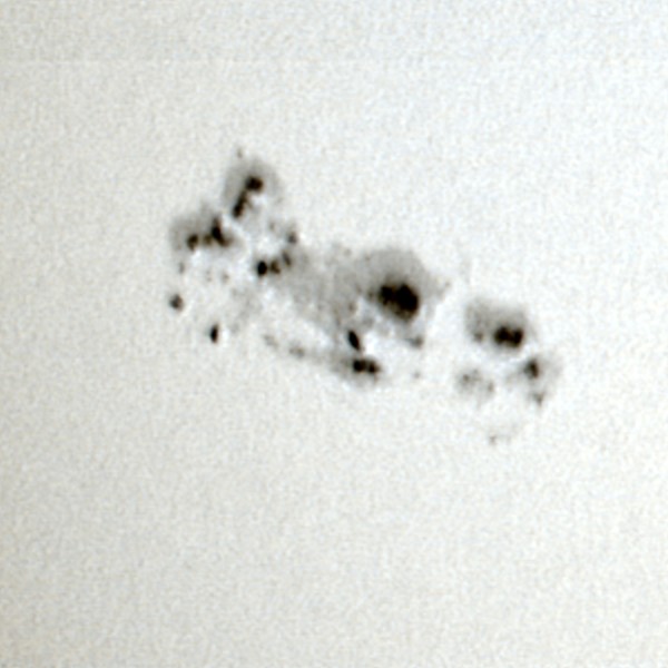 (Image from wikipedia)
Do you count only the very dark areas as sunspot, or the dark grey regions? If only the very dark areas (which is my supposition), or the larger dark grey areas? If the darker grey area, there will be significant issues of observability based on telescope quality. If the the very dark areas, do you count the the large extended region on the upper right of the group as one spot, because it is continuous , or as two because of the obvious necking between the left and right regions of the group? On a similar basis, do you count the long thin vertical dark region on the upper left as 1, 2 or 3 sunspots on a similar basis? Further, what of the very small dark spots on the within the darker background? Are they distinct sunspots, or just part of the general variation of darkness within that background?
Third, obviously the observational questions above are made more difficult for sunspot groups observed near the limb of the Sun, and also when observational conditions are poor due to weather (as sunspot observations are made by ground based telescopes).
Fourth, historically sunspot observations have not been complete. In particular, prior to 1849 up to twenty days may be missing from any given months observations.
To compensate for these issues, sunspots are measured by using the Wolf Number, which is K(10g+s), where g is the number of groups, and s is the number of sunspots observed.
g is multiplied by 10 because that is the average number of spots per group, but that is an obvious additional source of potential error when we take the Wolf number as a direct index of solar activity.
K is the "personal reduction coefficient":
(Source)
Although scaling by K is necessary for a consistent index, again it is a potential source of error.
Despite the scaling for groups and the use of a personal reduction coefficient introduces potential errors, by compensating for the other factors above, I assume they result in a smaller overall error in the index.
(Image from wikipedia)
Do you count only the very dark areas as sunspot, or the dark grey regions? If only the very dark areas (which is my supposition), or the larger dark grey areas? If the darker grey area, there will be significant issues of observability based on telescope quality. If the the very dark areas, do you count the the large extended region on the upper right of the group as one spot, because it is continuous , or as two because of the obvious necking between the left and right regions of the group? On a similar basis, do you count the long thin vertical dark region on the upper left as 1, 2 or 3 sunspots on a similar basis? Further, what of the very small dark spots on the within the darker background? Are they distinct sunspots, or just part of the general variation of darkness within that background?
Third, obviously the observational questions above are made more difficult for sunspot groups observed near the limb of the Sun, and also when observational conditions are poor due to weather (as sunspot observations are made by ground based telescopes).
Fourth, historically sunspot observations have not been complete. In particular, prior to 1849 up to twenty days may be missing from any given months observations.
To compensate for these issues, sunspots are measured by using the Wolf Number, which is K(10g+s), where g is the number of groups, and s is the number of sunspots observed.
g is multiplied by 10 because that is the average number of spots per group, but that is an obvious additional source of potential error when we take the Wolf number as a direct index of solar activity.
K is the "personal reduction coefficient":
(Source)
Although scaling by K is necessary for a consistent index, again it is a potential source of error.
Despite the scaling for groups and the use of a personal reduction coefficient introduces potential errors, by compensating for the other factors above, I assume they result in a smaller overall error in the index.


Comments