


 Arguments


Uncertainty, sensitivity and policy: Kevin Cowtan's AGU presentation
Posted on 15 January 2015 by Kevin C
The surface thermometer record forms a key part of our knowledge of the climate system. However it is easy to overlook the complexities involved in creating an accurate global temperature record from historical thermometer readings. If the limitations of the thermometer record are not understood, we can easily draw the wrong conclusions. I reevaluated a well known climate sensitivity calculation and found some new sources of uncertainty, one of which surprised me.
This highlights two important issues. Firstly the thermometer record (while much simpler than the satellite record) requires significant expertise in its use - although further work from the record providers may help to some extent. Secondly, the policy discussion, which has been centered on the so called 'warming hiatus', has been largely dictated by the misinformation context, rather than by the science.
At the AGU fall meeting I gave a talk on some of our work on biases in the instrumental temperature record, with a case study on the implications from a policy context. The first part of the talk was a review of our previous work on biases in the HadCRUT4 and GISTEMP temperature records, which I won't repeat here. I briefly discussed the issues of model-data comparison in the context of the CMIP-5 simulations, and then looked at a simple case study on the application of our results.
The aim of doing a case study using our data was to ascertain whether our work had any implications beyond the problem of obtaining unbiased global temperature estimates. In fact repeating an existing climate sensitivity study revealed a number of surprising issues:
- Climate sensitivity is affected by features of the temperature data which were not available to the original authors.
- It is also affected by features of the temperature record which we hadn't considered either, such as the impact of 19th century ship design.
- The policy implications of our work have little or nothing to do with the hiatus.
The results highlight the fact that significant expertise is currently required to draw valid conclusions from the thermometer record. This represents a challenge to both providers and users of temperature data.
Background
Let's start by looking at the current version of our temperature reconstruction, created by separate infilling of the Hadley/CRU land and ocean data. The notable differences are that our reconstruction is warmer in the 2000's (due to rapid arctic coverage), and around 1940, and cooler in the 19th century due to poor coverage in HadCRUT4 (figure 1).
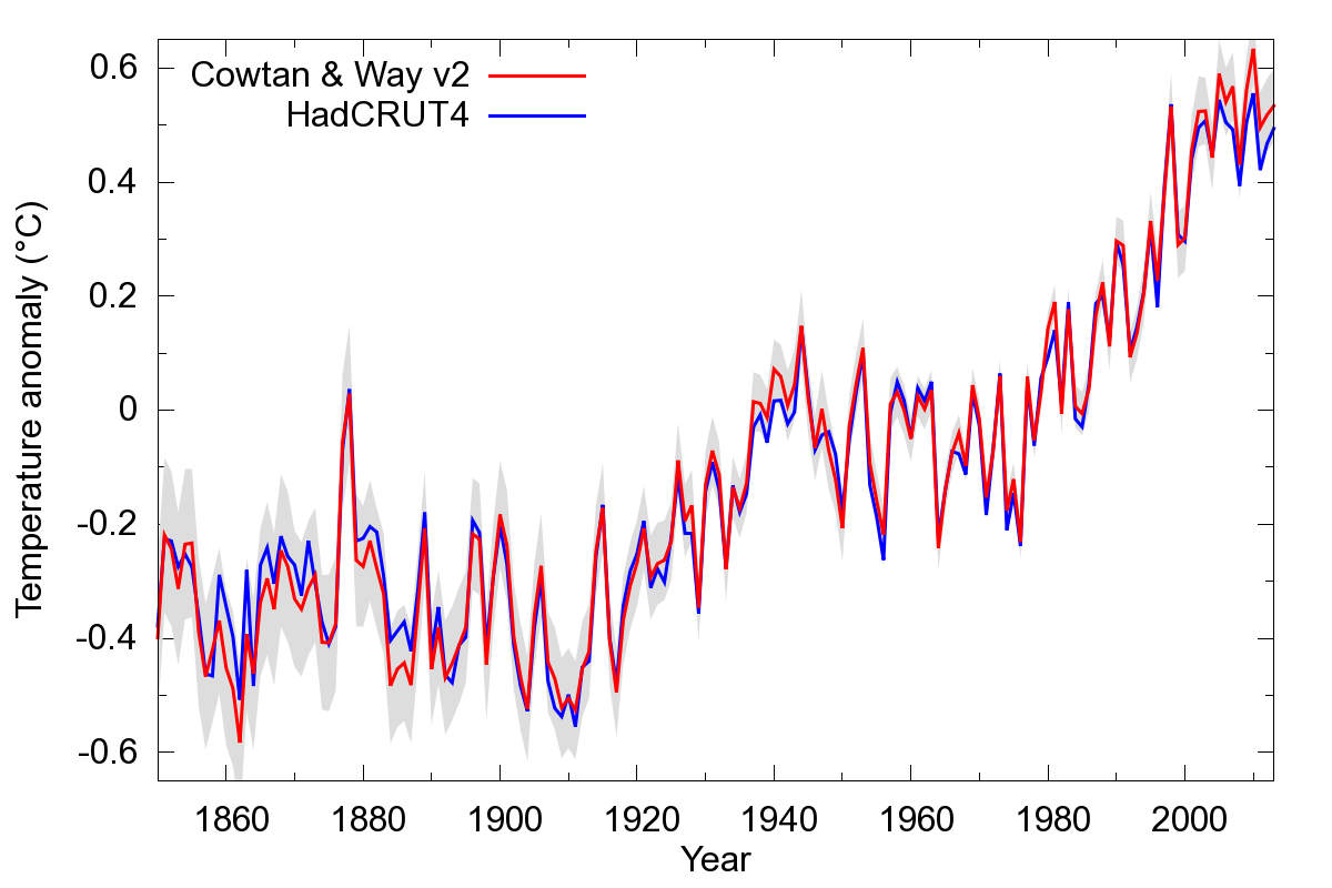
Figure 1: Comparison of the Cowtan and Way version 2 long reconstruction against HadCRUT4, showing the uncertainty interval from CWv2.
What impact do these differences have on our understanding of climate? The most important factor in determining the rate of climate change over our lifetimes is climate sensitivity, and in particular the Transient Climate Response (TCR). TCR measures how much global temperatures will change over a few decades due to a change in forcing, for example due to a change in greenhouse gas concentrations. It is therefore important from a policy perspective. We can look at the effect of our work on TCR estimates.
One widely reported estimate of TCR comes from a 2013 paper on climate sensitivity by Otto et al., from which figure 2(a) below is derived. The origin represents a reference period in the 19th century (specifically 1860-1879), while the data points represent the change in temperature (y-axis), against the forcing or driver or climate change (x-axis) for the 1970s, 1980s, 1990s and 2000s.
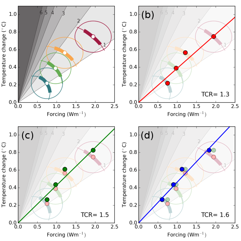
Figure 2: Estimates of Transient Climate Response (TCR) based on the method of Otto et al. (2013), reproducing the original calculation (b), with the introduction of the CWv2 temperature data (c) and with a thermal inertial term (d).
The slope of a line through these points gives an estimate how much temperature will change due to future changes in forcing. This is expressed in terms of the transient climate sensitivity (TCR), shown in figure 2(b). The Otto paper attracted some comment due to the TCR estimate being a little lower than is typically reported for climate models.
Note in particular the last datapoint, which lies almost on the line. The surface warming slowdown of the 2000s, commonly known as the 'hiatus', does not affect the estimate of climate sensitivity in the Otto et al. calculation.
How does our temperature reconstruction (Cowtan & Way 2014) affect this study? The answer is shown by the green points in figure 2(c). All the data points move upwards – this is actually due to the reference period in the 19th century being cooler in our data. The last data point moves further, reflecting the warmer temperatures in the 2000s. The transient climate sensitivity (TCR) increases accordingly.
One other feature of the Otto et al. calculation is that it ignores the thermal inertia of the system. In reality it takes a while for surface temperature to respond to a change in atmospheric composition: temperature change lags forcing. We can approximate this response by delaying the forcing a little (specifically by convolution with an exponential lag function with an e-folding time of 4 years, normalised to unit TCR). This gives the blue points in figure 2(d). The fit is a little better, and the TCR is now not far off from the models.
What factors are relevant to policy?
Does this solve the discrepancy between the models and the Otto et al. calculation? Unfortunately not. Shindell (2014) noted a more important issue – the impact of cooling particulate pollution (aerosols) on the radiative forcing in the Otto calculation is probably underestimated, due to the geographical distribution of the pollution. Underestimation of this cooling effect leads to an overestimation of the forcing and an underestimation of climate sensitivity. This is more important than the effects we identified: You can get pretty much any answer you like out of the Otto et al. calculation if you can justify a value for the aerosol forcing.
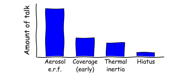
If we order the factors affecting climate sensitivity by their importance, the list probably looks like this:
- The size of the aerosol cooling effect.
- Coverage bias in the early temperature record.
- Thermal inertia.
- Hiatus factors (volcanoes, solar cycle and industrial emissions).
Put all of these together, and estimates of climate sensitivity from 20th century temperatures could exceed those from climate models. And given that transient sensitivity (TCR) is important for policy, we would expect political and public discourse to be dominated by those same factors:
Whereas in the real world, the public discourse looks more like this:
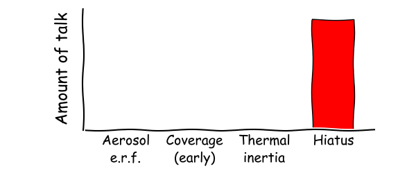
The public discourse does not reflect the science, rather it has been determined by the misinformation context. Some of this has crept back into the scientific discourse as well.
Naval architecture and climate sensitivity
Unfortunately that is not the end of the problems. So far we've largely ignored the oceans, which are quite important. By chance I was looking at a new sea surface temperature dataset, ERSST version 4, to determine what effect it might have on future versions of GISTEMP. What happens if we swap out the Hadley sea surface temperature data, and swap in the new version of ERSST (version 4)?
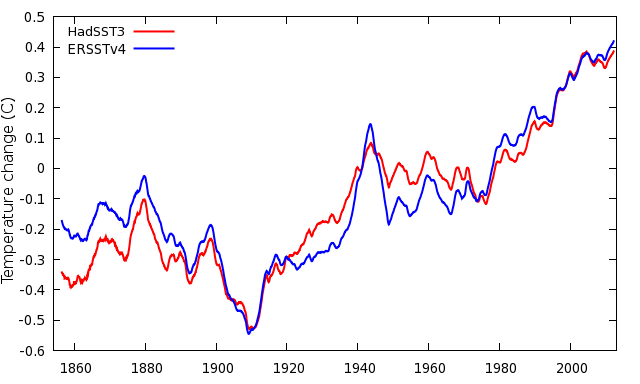
Figure 4: Comparison of HadSST3 and ERSSTv4 over map cells where both include values.
The two sea surface temperature series are shown in figure 4. When we use ERSSTv4 instead of HadSST3, two things happen:
- Recent temperature trends increase still further, because ERSSTv4 includes the correction for the transition from engine room intake to buoy observations. Using ERSSTv4 the 'hiatus' is a fairly insignificant affair.
- The climate sensitivity drops, due to warmer sea surface temperatures in the 19th century in ERSSTv4.
Why are the ERSSTv4 sea surface temperatures higher in the 19th century? The differences arise from a correction applied to early sea surface temperature observations. Early readings were taken by lifting water to the deck of a ship in a bucket, and measuring its temperature. The water cools during the process, leading to a bias which varies according to a number of factors, including the height of the ship's deck. ERSSTv4 does not show the expected decline in bucket correction with the lower ship deck heights in the 19th century. The bucket correction is large, so this could be a big effect, and yet I have never seen a climate paper discussing the impact of 19th century ship design on estimates of climate sensitivity.
The Otto et al. calculation addressed uncertainty in the temperature data by using the ensemble of temperature reconstructions provided by the UK Met Office. The Met Office HadCRUT4 data provide the most sophisticated representation of uncertainties currently available, but only encompasses uncertainty within the Met Office data and does not include uncertainties across the different temperature providers. Unfortunately there is no convenient way for users of temperature data to do this at the moment, especially if it involves mixing and matching temperature data across providers. This represents a significant weakness in current temperature data provision.
Fortunately, addressing this problem does lie within the remit of the International Surface Temperature Initiative (ISTI), so hopefully the situation will improve in the long run. In the meantime, I'd suggest the following rule of thumb when thinking about the accuracy of the thermometer record:
- Before 1880: Tentative (coverage is abysmal and the bucket correction highly uncertain)
- 1880-1960: Crude (coverage improving but no Antarctic stations, bucket correction uncertain)
- 1960-2000: Good (coverage good and sea surface temperatures largely consistent)
- 2000-now: Fair (coverage good but missing rapid Arctic warming, transition from ships to buoys)
The Otto et al. climate sensitivity calculation and others using 19th century temperatures as a baseline (for example Lewis and Curry 2014), are strongly dependent on the temperatures during the early and most problematic part of the record.
Summary
The instrumental temperature record is an important source of climate information, and when used with care can answer a great many questions. However the data are not without their problems, and their interpretation requires significant expertise in both the data and their limitations. Current provision does not make this as convenient for the user as it might be, however ongoing projects, and in particular the International Surface Temperature Initiative, will do much to address these issues.
The policy discussion however is oblivious to these questions, and revolves around issues like the slowdown in warming, which in practice has at most a minor impact on our climate sensitivity estimates and certainly less impact than uncertainty in the size of the aerosol cooling effect or the bucket corrections.


"The public discourse does not reflect the science, rather it has been determined by the misinformation context. Some of this has crept back into the scientific discourse as well."
It's that last bit that is particularly worrisome to me, particularly since that then feeds back into the denialosphere and they can and do say, "See, the scientists admitted that there's a 'pause'!" whenever anyone uses this terminology.
Very interesting point about 19th century bucket sampling. It seems to me that I have read some discussion of this issue, but I can't remember where, now.
Two or three quick points.
1) The authors of Otto et al (who include myself as well as fourteen lead authors of parts of the IPCC AR5 WG1 relevant to TCR and ECS [equilibrium climate sensitivity] estimation) were not mistaken in ignoring the thermal inertia of the climate system when estimating TCR. TCR is defined on a basis which does not account for that thermal inertia. So the estimate in Figure 2(d) is on a different basis than that which corresponds to TCR, and is bound to overstate TCR. I imagine that the same mistake was made in the recent paper by Cawley et al. when estimating TCR using their Alternative minimal model.
2) Well done for highlighting that the hiatus is not of any real significance for estimates of TCR and ECS. Many clmate scientists fail to understand this point - e.g., see Rogelj et al. (2014). As you state, the greatest source of uncertainty is aerosol forcing (ERF).
3) As I've pointed out to Robert Way before, the difference between the amount of warming over the instrumental period shown by HadCRUT4 and the Cowtan & Way infilled reconstruction based thereon appears to be largely due the way temperatures over sea ice are treated rather than a lack of high latitude coverage in HadCRUT4 per se. The global temperature rise from 1860-79 to 1990-99 per HadCRUT4 (v2 or v3) is virtually identical to the BEST reconstruction with sea temperature used for infilling where there is sea ice. Using air temperatures for infilling where there is sea ice, as the other version of BEST and Cowtan & Way reconsruction do, produces a temperature rise about 6% greater.
Nic Lewis @2, the definition of "Transient Climate Response" (TCR) is given by the IPCC as follows:
As CO2 has not increased by 1% per annum, is not the only forcing change, and we cannot measure ten years into the future to get the 20 year period, not empirical measurement is the TCR, and certainly not by definition. You may think you have defined the TCR as F2xΔT/ΔF (where F2x is the forcing for doubled CO2, ΔT is the change in temperature, and ΔF is the change in forcing). You have not. Rather you have taken the current temperature response to the change in forcing to be a convenient approximation to the TCR.
Given that your formula (2) from Otto et al (2013) is an estimator of TCR, not a definition, it is quite possible as a matter of empirical fact that it is a poor estimator, or that an estimator taking into account thermal inertia is superior.
[Rob P] - inflammatory text deleted. Please stick to the science and dial the tone down. Thanks.
Nic Lewis at 09:19 AM on 16 January, 2015
"3) As I've pointed out to Robert Way before, the difference between ... HadCRUT4 and the Cowtan & Way ... appears to be largely due the way temperatures over sea ice are treated rather than a lack of high latitude coverage in HadCRUT4 per se. The global temperature rise from 1860-79 to 1990-99 per HadCRUT4 (v2 or v3) is virtually identical to the BEST reconstruction with sea temperature used for infilling where there is sea ice. Using air temperatures for infilling where there is sea ice, as the other version of BEST and Cowtan & Way reconsruction do, produces a temperature rise about 6% greater"
Nic Lewis,
Running your code with CW2014 as opposed to HadCRUTv4.2 increases the TCR from 1.33 to 1.47 which corresponds to a ~10% increase in TCR using your method.
Secondly, and more importantly, a thorough read of Cowtan and Way (2014) would show that air temperatures over sea ice should be treated in the same manner as land and not SSTs. You are also welcome to read Dodd et al (2014) and Simmons and Poli (2014) which each find general agreement with the approach we employ. You might also recognize that drift stations on the ice were used in validation of the approach in Cowtan and Way (2014) and these have supported the sea ice treated as land approach. It makes physical sense to those of us who have spent a fair amount of time in the Arctic. This has all been previously pointed out to you.
Nic Lewis,
I should also mention that Comiso and Hall (2014);s AVHRR satellite skin temperature data and our tests with AIRS satellite data (see our supplementary documents we have uploaded on our website) both support the results of CW2014. Your argument, pardon the pun, is on thin ice.
The issue of how to handle air temperatures over sea ice was in fact the most difficult question we faced. However that's not because there's any uncertainty in the answer - theory, observations, models and expert opinion all point the same way - it's just because no-one has collected all the evidence in one place before. I probably ought to write it up as a paper. I'll try and write a summary in this thread later today, but it's going to be quite long.

But here's one little result I've got pre-prepared. Here's a comparison of CWv2 against ERA-i and MERRA for the region N of 70N:
There's quite a lot of agreement there. Note that the reanalyses show 1998 as even cooler than we do, which would increase the trend since 1998 further.
The only big difference is the period 2010-2012, which MERRA shows as rather cooler, although they come back into line for recent years. What could that be?
The most obvious difference between MERRA and the other two is that MERRA doesn't use land station temperatures - only pressures. So my first thought was to look for a land station homogenisation problem. However, the data argue against that:
1. The difference between MERRA and ERA is seasonal - it only occurs in winter. (In fact all the warming occurs in winter, because in summer melting anchors the temperatures around zero). Station homogenization problems tend to involve jumps, not seasonal differences.
2. The difference isn't localised over a weather station. In fact it's concentrated in the central arctic in a region whose shape matches the region which is most distant from any weather station.
Given that we've already seen that MERRA can show large spurious trends in Africa for regions isolated from the nearest SST or barometer (see our 3rd update), then the current working hypothesis is that MERRA is at fault here. I haven't looked at JMA, but Simmons and Poli (2014) suggests that it is closer to ERA-i. The ERA temperatures also make more sense in terms of the 2012 sea ice minimum than MERRA.
One other feature of interest: Arctic temperatures (and hence the Arctic contribution to coverage bias) have largely stablised since 2005. The big change is from 1997-2005. From this and from looking at similar behaviour in climate models, I do not think that we should assume continued rapid arctic warming, or an early disappearance of Arctic sea ice. My currect working hypothesis is that the models are right when it comes to an ice free Arctic.
James Hansen has argued for decades that a satalite capable of measuring aerosols is desperately needed to measure the affect on climate sensitivity. Unfortunately, the mission with that capability was destroyed on launch a few years ago. Does anyone know the status of a replacement satalite?
Why does NASA put so much effort into Mars when holes in their data like this still exist?
This is a very brief outline. It's late and I'm tired, so apologies for the poor writing:
Why do we reconstruct temperatures over sea ice from land temperatures? There are four sources of evidence on which this decision was made:
But first, one thing needs to be clear: rapid arctic warming is a winter phenomena. The central arctic can't warm in summer, because melting ice holds the temperature around zero. That's vital to understand the rest of this discussion - we are talking about something which happens in winter.
The physics
Global mean surface temperature is based on historical records, which limit how we can measure it. We can't use brightness temperatures because we don't have the data. We've got weather station data, so we use 2m air temperatures. But marine air temperatures are unreliable, so we use sea surface temperature as a proxy for air temperature over the oceans.
When it comes to understanding the physics of the problem, to a first approximation we can say that the sun heats the surface and the surface heats the air. If the surface is cool, it can cool the air too. That's true for land or ocean.
The big difference is that ocean surface is liquid, and surface mixing means that the effective surface heat capacity is much greater than for land. (Waves and spray improve heat exchange with the air too). As a result, temperature variation over land is much greater than over the oceans, whether it be diurnal or seasonal. Many of us experience this if we visit the coast - temperatures swings become smaller as you approach the sea.
What happens over sea ice? The air temperature is no longer coupled to the water temperature. Ice is a reasonable insulator, and snow on ice is very good (Kurtz et al 2011). So the thing which makes oceans different from land has gone away. Air temperatures over water behave differently from air temperatures over land. Air temperatures over sea ice, especially with a covering of snow, behave like air temperatures over land.
This different behaviour can be seen in the land and ocean temperature data. They show different amounts of variation over time, and they vary spatially over different distances. And if we use the land and ocean data to reconstruct temperatures in the isolated central arctic, we get very different results - mainly because of the different behaviour of the temperatures fields (but the distance to the nearest observation plays a role too).
The models
The reanalysis models incorporate the physics, including freezing/melting effects. And as we saw in my last post, the three modern models agree well with our reconstruction. Here's a month-by-month comparison to MERRA, comparing kriging reconstructions from the land and ocean data respectively. This is for the most isolated region of the central arctic, chosen to be most distant from any weather station, and so it's as hard as it gets. The SST based reconstruction doesn't show remotely enough variation, whereas the land data shows the right sort of variability, and fairly good agreement with the features even for the most isolated region of the Arctic.
Observations
In the paper we did a comparison over the same region with the international arctic buoy program (IABP) data of Rigor et al. In particular they produced a dataset by kriging combining land stations and temperatures measured on ice buoys in the central arctic. We showed a comparison with IABP in the paper. Rigor et al also examined kriging ranges by season, and found that while the distances over which temperatures were correlated in the summer were small, in winter they could be up to 1000km, including between land and ice stations.
In addition, the AVHRR satellite data also show rapid arctic warming comparable to reanalysis models. So there are two independent source of observational data showing similar behaviour over ice to us.
The experts
Because I was worried about this issue, I went to the 2013 EarthTemp meeting on temperatures in the Arctic. Which meant I could ask the experts about how air temperatures behave over sea ice. And they produced the same answer, for basically the theoretical reasons I outlined above.
Practical aspects
So what would happen if we were to reconstruct temperatures over the central arctic from sea surface temperatures instead of from air temperatures?
Winter sea ice extent hasn't changed as much as summer extent, which means that the limit of the winter sea ice hasn't moved very far. Sea surface temperatures at the edge of the sea ice are anchored at around freezing for the same reason as arctic temperatures in the summer. Further away from the ice other factors, such as tropic sea surface temperature and meridional heat transport also play a role. Even so, the variation in sea surface temperature in the northernmost sea cells in winter is small, and as a result a reconstruction from sea surface temperature will never show much change.
In other words, if we reconstruct air temperatures over sea ice from sea surface temperatures, we are imposing a constraint that the central arctic can not change in temperature, even in winter. But we're doing so with no physical basis - the freezing of water more than 1500km away doesn't constrain temperatures, any more than sea surface temperatures can do much to moderate temperature extremes 1500km inland.