


 Arguments


How curve-fitting can ignore physics
What the science says...
Loehle and Scafetta's paper is nothing more than a curve fitting exercise with no physical basis using an overly simplistic model.
Loehle and Scafetta find a 60 year cycle causing global warming
About 60% of the warming observed from 1970 to 2000 was very likely caused by this natural 60-year climatic cycle during its warming phase...climate may remain approximately steady until 2030-2040, and may at most warm 0.5-1.0°C by 2100 at the estimated 0.66°C/century anthropogenic warming rate, which is about 3.5 times smaller than the average 2.3°C/century anthropogenic warming rate projected by the IPCC during the first decades of the 21st century (Craig Loehle)
In a paper published in The Bentham Open Atmospheric Science Journal, which has received a significant amount of blogosphere attention (for example, with posts published on the "skeptic" blogs of Judith Curry and Anthony Watts), two "skeptics", Loehle and Scafetta (L&S), performed the same sort of curve fitting exercise using a simple model of the climate.
Usually in climate modeling, scientists will set the allowable range for each input parameter based on observational data. For example, the ocean mixed layer, in which the density is approximately the same as the ocean surface, is at most between 25 and 200 meters (generally more like 50-100 meters). Once they have established these ranges, climate scientists can run the climate models and compare their results to recent observational data (a.k.a. "hindcasting"), and tweak the models (within the physically allowable ranges) to match the observational data.
This is not how the "skeptics" do modeling. For example, Spencer has previously used a mixed ocean layer depth of 700 meters, because although this is physically unjustifiable, it allowed his model to fit the data with a low climate sensitivity. In this case, L&S use a model with a very simple formula:
You may be able to guess how their model will perform just by examining this formula. The first two terms are oscillations of 60 and 20 year periods, respectively. The third term will produce a linear warming trend, and the fourth is simply a constant. So this model will produce a linear warming trend with two natural oscillations superimposed on top of it. L&S tweaked the parameters to fit the temperature curve without doing any further testing, but we can test it for them by running their model backwards in time and comparing to reconstructed temperatures. Because of the linear term, you might expect the model to match the observations back to the Little Ice Age (LIA) and then rapidly diverge from observations. If so, you would essentially be right (Figure 1).
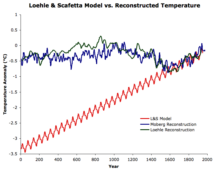
Figure 1: The L&S Case 2 model projected backwards in time (red), compared to the Moberg et al. (2005) millennial northern hemisphere temperature reconstruction (blue) and the Loehle (2008) millennial global temperature reconstruction (green).
Talk about a divergence problem!
Loehle is generally most well-known for his millennial global temperature reconstruction using non-tree ring proxies. Although the paper was published in Energy & Environment, which is not considered a peer-reviewed journal, considering that Loehle was the lead author on L&S, we felt it would be worthwhile to see if Loehle's model matches his own temperature reconstruction.
The L&S model matches the reconstructed temperature trends reasonably well back to the 17th century, but fails miserably to match prior temperatures. Moreover, the 60 year cycle in the L&S model matches up extremely poorly with the Moberg reconstruction (Figure 2), and even with Loehle's own reconstruction (Figure 3).
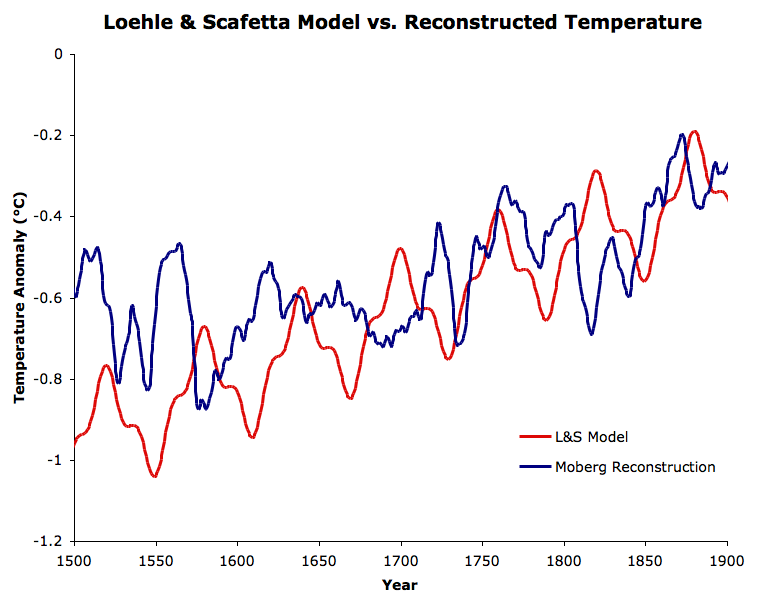
Figure 2: The L&S Case 2 model projected backwards to the period 1500 to 1900, compared to the Moberg et al. (2005) milennial northern hemisphere temperature reconstruction.
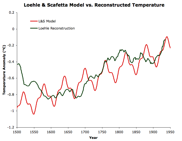
Figure 3: The L&S Case 2 model projected backwards to the period 1500 to 1900, compared to the Loehle (2008) milennial global temperature reconstruction.
Several times between 1500 and 1900, the L&S model is anti-phase with both reconstructions, with the peak of the 60 year cycle matching a trough in temperature. Thus we see that although L&S have gotten lucky and matched the temperature trend a few centuries into the past, the 60 year cycle which is the basis of their paper is nowhere to be found in the temperature data.
Why Does the L&S Model Fail the Hindcasting Test?
So why the hindcasting failure? The basic reason is simple - this is not a physical model. L&S describe their methodology in the paper:
"The model was fit by nonlinear least squares estimation using Mathematica functions, with phase and amplitude free but period fixed as above."
In other words, they let the parameters vary freely without any physical constraints, and fit the curve as best they could. They suggest the first two terms represent astronomical cycles:
"The solar system oscillates with a 60-year cycle due to the Jupiter/Saturn three-synodic cycle and to a Jupiter/Saturn beat tidal cycle"
How exactly these Jupiter and Saturn orbital cycles are supposed to impact the Earth's surface temperature is left unexplained, and thus there are no realistic physical constraints on their parameters 'A' and 'B', which correspond to the amplitude of the cyclical effects on global surface temperature. Is it realistic for a Jupiter/Saturn cycle to have an effect on the Earth's average temperature with an peak-to-trough amplitude of 0.24°C? It seems exceptionally unlikely, but this question is left unanswered, and thus the model has no physical basis (more on these astronomical cycles below).
Linear Trends and Bad Assumptions
But the real L&S model failure is in the linear trend, since these mysterious astronomical cycles are simply oscillations on top of that trend. Actually, in the paper, L&S apply two different cases to their model. In Case 1, they simply apply it to the observational data from 1850 to 2010. L&S are able to achieve a decent fit with Case 1, but conclude that the residual (subtracting model output from observations) is non-random, and thus they're missing some key components.
They then try "Case 2", in which they fit their model from 1850 to 1950 (but apply it through 2010), and then apply an additional linear trend from 1950 to 2010, which they claim is the man-made global warming signal. They assume that humans have zero influence on the global surface temperature prior to about 1950, which is a poor assumption.
A second problem is that L&S do not evaluate whether the remaining residual after they apply the second (anthropogenic) linear trend is random - it appears not to be (see their Figure 2b, the lower graph in our Figure 4):
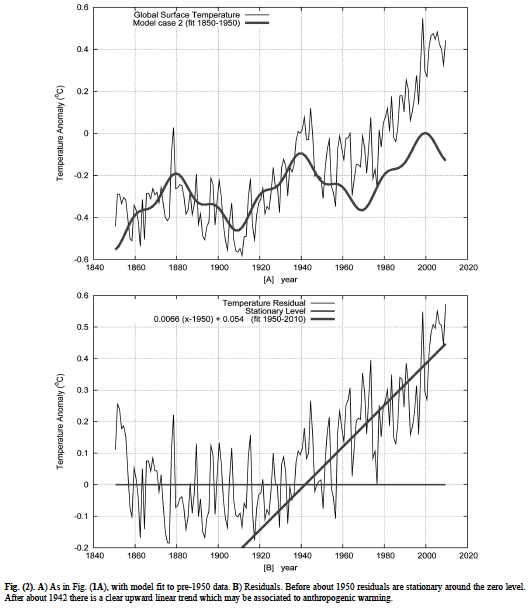
Figure 4: L&S Case 2 Model vs. HadCRUT global surface temperature (upper frame), residual plus a linear trend fitting data from 1950 to 2010, representing the man-made warming effect (lower frame).
Quite possibly the biggest flaw in the paper (and there are many to choose from), is in their "natural" linear trend, which L&S describe thusly:
"The linear trend would approximately extrapolate a natural warming trend due to solar and volcano effects that is known to have occurred since the Little Ice Age"
Other than the supposed man-made linear trend L&S apply in Case 2 starting in 1950, and the two cyclical factors which cause zero long-term trend, this "natural" linear trend is the only factor included in the L&S model. In other words, it must account for every non-cyclical "natural" effect (forcing) on the average global temperature.
So why do L&S assume natural forcings have had a constant warming effect over the past 160 years? They provide no justification for this assumption, and it is clearly faulty. For example, solar activity increased significantly in the early 20th century, but has remained essentially flat (even declining slightly) since 1950. Meehl et al. (2004) provide a graph of the natural forcings over the period in question (Figure 5).
Figure 5: Natural radiative forcings from Meehl et al. (2004)
Quite clearly the natural radiative forcing does not increase at a constant linear rate from 1850 to 2010, and thus the assumption which is the backbone of the L&S model is faulty. By overestimating the "natural" contribution to the 1950-2010 warming, they necessarily underestimate the human contribution, and thus underestimate the climate sensitivity to increasing CO2 (more on this later).
Since the L&S model is so oversimplified, failing to account for changes in the natural forcings, they fail to accurately model past climate changes. For the same reason, they will fail to accurately model future climate changes as well.
Astronomical Cycles
Another fundamental problem with the L&S model is the assumption of significant effects of 20 and 60 year astronomical cycles on the Earth's temperature. Aside from failing to provide a physical mechanism through which Jupiter and Saturn could impact the Earth's temperature, as Riccardo has previously noted, the mere existence of a 60 year cycle in the Earth's surface temperature depends on the choice of trend to begin with. By fitting certain polynomials to the global temperature data, we can find a residual with a 60 year cycle, but only with certain curve fitting choices. Those curve fitting choices must first be justified.
However, instead of first subtracting off the underlying trend and seeing what's left, L&S start their exercise under the assumption that the 20 and 60 year cycles are present, and then fit the temperature data as best they can with those cycles (with no physical constraints). After they conduct this curve fitting, they see what's left and attribute the remainder to human effects. This is not a scientific approach, it's simply curve fitting (a.k.a. "graph cooking" and "mathturbation") at its worst.
There may be a 60 year cycle in the global climate, perhaps related to an oceanic cycle like the Pacific Decadal Oscillation. However, in order to explain the warming of both the oceans and atmosphere, there must be an external forcing at work, which may be why L&S invoke these mysterious astronomical cycles. But the fact remains that they have failed to provide a physical mechanism through which these cycles could impact the Earth's climate. And as we saw in Figures 2 and 3, their assumed 60 year cycle does not show up in millennial temperature reconstructions - not even in Loehle's own previous work! This is a rather glaring contradiction.
Aerosols
The effects of aerosols on the climate are a problem for the L&S model, as the authors almost admit in the paper:
"Residual analysis does not provide any evidence for a substantial cooling effect due to sulfate aerosols from 1940 to 1970....sulfate aerosols produced by volcanoes or industrial emissions no doubt have a cooling effect"
We have recently discussed several papers which have found substantial global dimming as a result of increased human aerosol emissions from 1950 to 1980 and 2000 to 2010. As L&S admit, this global dimming due to aerosols "no doubt [has] a cooling effect", yet it doesn't show up in their model. This is further evidence of the unconstrained overfitting of their 20 and 60 year cycles.
Future Warming Prediction Flaws
As noted above, since the L&S model fails the hindcasting test, there is no reason to believe it can accurately predict future global temperature changes. However, that's not the only problem with their prediction. The authors also assume that the linear man-made warming trend which they've thrown into their model will continue at the same linear rate into the future. We have previously addressed this misconception in Monckton Myth #3: Linear Warming. The only way we will prevent man-made warming from accelerating is if we take significant action to reduce our greenhouse gas emissions, which "skeptics" generally oppose. L&S don't even provide the emissions scenario for their future warming prediction - they simply assume that the linear man-made warming trend will continue without any justification. Once again, this is a glaring lack of physics in their paper.
Climate Sensitivity Estimate Flaws
L&S estimate the equilibrium climate sensitivity to doubled CO2 from their model at "about 1-1.5°C or less". However, there are two major problems with this estimate:
- As noted above, L&S have overestimated the 'natural' warming effects from 1950 to 2010, and as a result, have underestimated the man-made warming effects over this period. Their climate sensitivity estimate is based entirely on this underestimated man-made warming trend, and thus is also too low.
- L&S are estimating an equilibrium climate sensitivity for a climate which is not currently in equilibrium. What they are actually trying to estimate here is the transient climate sensitivity, but they erroneously compare it to the IPCC equilibrium sensitivity range.
The Bentham Open Journals
At this point, you may be wondering how such a tremendously flawed paper made it through the peer review process. The paper was published in the Bentham Open Atmospheric Science journal. The Bentham Open journals appear to have a tendency to publish 'controversial' papers which most peer-reviewed journals would not publish. There has also been a case of another Bentham Open journal accepting a nonsensical hoax submission paper, which calls the peer-review standards of these journals into question. Additionally, the ISI Master Journal list does not recognize the Bentham Open journals as legitimately peer-reviewed.
The paper should be evaluated on its own merits, of course (which are basically non-existent), but the publication of this paper probably had a lot to do with the low standards and quality of peer-review of the journal in which it was published.
Nothing to See Here
Unfortunately, there is little we can learn from the L&S paper. Fitting a curve with a simple model using physically unconstrained parameters is simply not a scientific process, as illustrated in its failure when put to the hindcasting test. You could just as easily conduct this sort of curve fitting exercise using the number of pirates, canoes, and pantaloons in southern Spain. L&S are guilty of a major error in the abstract of their paper:
"About 60% of the warming observed from 1970 to 2000 was very likely caused by the above natural 60-year climatic cycle during its warming phase."
Correlation is not causation; all L&S have demonstrated in their unphysical curve fitting exercise is a correlation between their cycles and global temperature. If I find a correlation between Spanish pirates and pantaloons and global temperature, that doesn't mean these variables are causing global warming. If you want to draw a conclusion like L&S have, you need to identify the physical mechanism through which your variables are causing a global temperature change, identify a realistic physical range that this effect can have on the temperature, and then run your model.
Without a realistic physical basis, like Spencer before them, all L&S are doing is playing pointless curve fitting games, and using their results to draw unsubstantiated conclusions.
Last updated on 1 August 2011 by dana1981.


Climate Myth...