


 Arguments


The anthropogenic global warming rate: Is it steady for the last 100 years? Part 2.
Posted on 7 May 2013 by KK Tung
This is part 2 of a guest post by KK Tung, who requested the opportunity to respond to the SkS post Tung and Zhou circularly blame ~40% of global warming on regional warming by Dumb Scientist (DS).
In this second post I will review the ideas on the Atlantic Multidecadal Oscillation (AMO). I will peripherally address some criticisms by Dumb Scientist (DS) on a recent paper (Tung and Zhou [2013] ). In my first post, I discussed the uncertainty regarding the net anthropogenic forcing due to anthropogenic aerosols, and why there is no obvious reason to expect the anthropogenic warming response to follow the rapidly increasing greenhouse gas concentration or heating, as DS seemed to suggest.
For over thirty years, researchers have noted a multidecadal variation in both the North Atlantic sea-surface temperature and the global mean temperature. The variation has the appearance of an oscillation with a period of 50-80 years, judging by the global temperature record available since 1850. This variation is on top of a steadily increasing temperature trend that most scientists would attribute to anthropogenic forcing by the increase in the greenhouse gases. This was pointed out by a number of scientists, notably by Wu et al. [2011] . They showed, using the novel method of Ensemble Empirical Mode Decomposition (Wu and Huang [2009 ]; Huang et al. [1998] ), that there exists, in the 150-year global mean surface temperature record, a multidecadal oscillation. With an estimated period of 65 years, 2.5 cycles of such an oscillation was found in that global record (Figure 1, top panel). They further argued that it is related to the Atlantic Multi-decadal Oscillation (AMO) (with spatial structure shown in Figure 1, bottom panel).
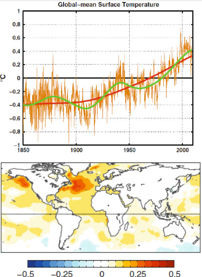
Figure 1. Taken from Wu et al. [2011] . Top panel: Raw global surface temperature in brown. The secular trend in red. The low-frequency portion of the data constructed using the secular trend plus the gravest multi-decadal variability, in green. Bottom panel: the global sea-surface temperature regressed onto the gravest multi-decadal mode.
Less certain is whether the multidecadal oscillation is also anthropogenically forced or is a part of natural oscillation that existed even before the current industrial period.
It is now known that the AMO exists in coupled atmosphere-ocean models without anthropogenic forcing (i.e. in “control runs”, in the jargon of the modeling community). It is found, for example in a version of the GFDL model at Princeton, and the Max Planck model in Germany. Both have the oscillation of the right period. In the models that participated in IPCC’s Fourth Assessment Report (AR4), no particular attempt was given to initialize the model’s oceans so that the modeled AMO would have the right phase with respect to the observed AMO. Some of the models furthermore have too short a period (~20-30 years) in their multidecadal variability for reasons that are not yet understood. So when different runs were averaged in an ensemble mean, the AMO-like internal variability is either removed or greatly reduced. In an innovative study, DelSol et al. [2011] extract the spatial pattern of the dominant internal variability mode in the AR4 models. That pattern (Figure 2, top panel) resembles the observed AMO, with warming centered in the North Atlantic but also spreading to the Pacific and generally over the Northern Hemisphere (Delworth and Mann [2000] ).
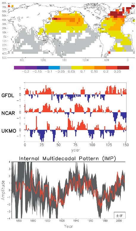
Figure 2. Taken from DelSol et al. [2011] . Top panel: the spatial pattern that maximizes the average predictability time of sea-surface temperature in 14 climate models run with fixed forcing (i.e. “control runs”). Middle panel: the time series of this component in three representative control runs. Bottom panel: time series obtained by projecting the observed data onto the model spatial pattern from the top panel. The red curve in the bottom panel is the annual average AMO index after scaling.
When the observed temperature is projected onto this model spatial pattern, the time series (in Figure 2 bottom panel) varies like the AMO Index (Enfield et al. [2001] ), even though individual models do not necessarily have an oscillation that behaves exactly like the AMO Index (Figure 2, middle panel).
There is currently an active debate among scientists on whether the observed AMO is anthropogenically forced. Supporting one side of the debate is the model, HadGEM-ES2, which managed to produce an AMO-like oscillation by forcing it with time-varying anthropogenic aerosols. The HadGEM-ES2 result is the subject of a recent paper by Booth et al. [2012] in Nature entitled “Aerosols implicated as a prime driver of twentieth-century North Atlantic climate variability”. The newly incorporated indirect aerosol effects from a time-varying aerosol forcing are apparently responsible for driving the multi-decadal variability in the model ensemble-mean global mean temperature variation. Chiang et al. [2013] pointed out that this model is an outlier among the CMIP5 models. Zhang et al. [2013] showed evidence that the indirect aerosol effects in HadGEM-ES2 have been overestimated. More importantly, while this model has succeeded in simulating the time behavior of the global-mean sea surface temperature variation in the 20th century, the patterns of temperature in the subsurface ocean and in other ocean basins are seen to be inconsistent with the observation. There is a very nice blog by Isaac Held of Princeton, one of the most respected climate scientists, on the AMO debate here. Held further pointed out the observed correlation between the North Atlantic subpolar temperature and salinity which was not simulated with the forced model: “The temperature-salinity correlations point towards there being a substantial internal component to the observations. These Atlantic temperature variations affect the evolution of Northern hemisphere and even global means (e.g., Zhang et al 2007). So there is danger in overfitting the latter with the forced signal only.”
The AMOC and the AMO
The salinity-temperature co-variation that Isaac Held mentioned concerns a property of the Atlantic Meridional Overturning Circulation (AMOC) that is thought to be responsible for the AMO variation at the ocean surface. This Great Heat Conveyor Belt connects the North Atlantic and South Atlantic (and other ocean basins as well), and between the warm surface water and the cold deep water. The deep water upwells in the South Atlantic, probably due to the wind stress there (Wunsch [1998] ). The upwelled cold water is transported near the surface to the equator and then towards to the North Atlantic all the way to the Arctic Ocean, warmed along the way by the absorption of solar heating. Due to evaporation the warmed water from the tropics is high in salt content. (So at the subpolar latitudes of the North Atlantic, the salinity of the water could serve as a marker of where the water comes from, if the temperature AMO is due to the variations in the advective transport of the AMOC. This behavior is absent if the warm water is instead forced by a basin wide radiative heating in the North Atlantic.) The denser water sinks in the Arctic due to its high salt content. In addition, through its interaction with the cold atmosphere in the Arctic, it becomes colder, which is also denser. There are regions in the Arctic where this denser water sinks and becomes the source of the deep water, which then flows south. (Due to the bottom topography in the Pacific Arctic most of the deep water flows into the Atlantic.) The Sun is the source of energy that drives the heat conveyor belt. Most of the solar energy penetrates to the surface in the tropics, but due to the high water-vapor content in the tropical atmosphere it is opaque to the back radiation in the infrared. The heat cannot be radiated away to space locally and has to be transported to the high latitudes, where the water vapor content in the atmosphere is low and it is there that the transported heat is radiated to space.
In the North Atlantic Arctic, some of the energy from the conveyor belt is used to melt ice. In the warm phase of the AMO, more ice is melted. The fresh water from melting ice lowers the density of the sinking water slightly, and has a tendency to slow the AMOC slightly after a lag of a couple decades, due to the great inertia of that thermohaline circulation. A slower AMOC would mean less transport of the tropical warm water at the surface. This then leads to the cold phase of the AMO. A colder AMO would mean more ice formation in the Arctic and less fresh water. The denser water sinks more, and sows the seed for the next warm phase of the AMO. This picture is my simplified interpretation of the paper by Dima and Lohmann [2007] and others. The science is probably not yet settled. One can see that the physics is more complicated than the simple concept of conserved energy being moved around, alluded to by DS. The Sun is the driver for the AMOC thermohaline convection, and the AMO can be viewed as instability of the AMOC (limit cycle instability in the jargon of dynamical systems as applied to simple models of the AMOC).
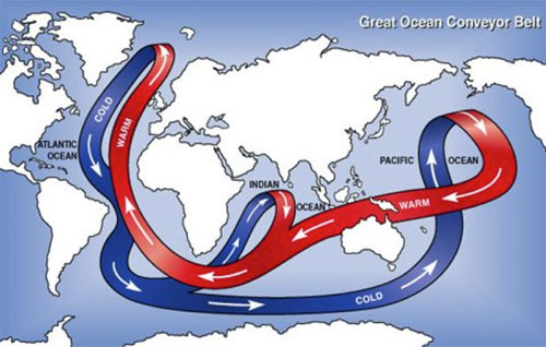
Figure 3. The great ocean conveyor belt. Schematic figure taken from Wikipedia.
Preindustrial AMO
It is fair to conclude that no CMIP3 or CMIP5 models have successfully simulated the observed multidecadal variability in the 20th century using forced response. While this fact by itself does not rule out the possibility of an AMO forced by anthropogenic forcing, it is not “unphysical” to examine the other possibility, that the AMO could be an internal variability of our climate system. Seeing it in models without anthropogenic forcing is one evidence. Seeing it in data before the industrial period is another important piece of evidence in support of it being a natural variability. These have been discussed in our PNAS paper. Figure 4 below is an updated version (to include the year 2012) of a figure in that paper. It shows this oscillation extending back as far as our instrumental and multi-proxy data can go, to 1659. Since this oscillation exists in the pre-industrial period, before anthropogenic forcing becomes important, it plausibly argues against it being anthropogenically forced.
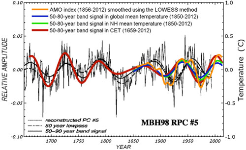
Figure 4. Comparison of the AMO mode in Central England Temperature (CET) (red) and in global mean (HadCRUT4) (blue), obtained from Wavelet analysis, with the multi-proxy AMO of Delworth and Mann [2000] (in thin black line). The amplitude of multi-proxy data is only relative (left axis). The orange curve is a smoothed version of the AMO index originally available in monthly form.
The uncertainties related to this result are many, and these were discussed in the paper but worth highlighting here. One, there is no global instrumental data before 1850. Coincidentally, 1850 is considered the beginning of the industrial period (the Second Industrial Revolution, when steam engines spewing out CO2 from coal burning were used). So pre-industrial data necessarily need to come from nontraditional sources, and they all have problems of one sort of the other. But they are all we have if we want to have a glimpse of climate variations before 1850. The thermometer record collected at Central England (CET) is the longest such record available. It cannot be much longer because sealed liquid thermometers were only invented a few years earlier. It is however a regional record and does not necessarily represent the mean temperature in the Northern Hemisphere. This is the same problem facing researchers who try to infer global climate variations using ice-core data in the Antarctica. The practice has been to divide the low-frequency portion of that polar data by a scaling factor, usually 2, and use that to represent the global climate. While there has been some research on why the low-frequency portion of the time series should represent a larger area mean, no definitive proof has been reached, and more research needs to be done. We know that if we look at the year-to-year variations in winters of England, one year could be cold due to a higher frequency of local blocking events, while the rest of Europe may not be similarly cold. However, if England is cold for 50 years, say, we know intuitively that it must have involved a larger scale cooling pattern, probably hemispherically wide. That is, England’s temperature may be reflecting a climate change. We tried to demonstrate this by comparing low passed CET data and global mean data, and showed that they agree to within a scaling factor slightly larger than one. England has been warming in the recent century, as in the global mean. It even has the same ups and downs that are in the hemispheric mean and global mean temperature (see Figure 4).
In the pre-industrial era, the comparison used in Figure 4 was with the multiproxy data of Delworth and Mann [2000]. These were collected over geographically distributed sites over the Northern Hemisphere, and some, but very few, in the Southern Hemisphere. They show the same AMO-like behavior as in CET. CET serves as the bridge that connects preindustrial proxy data with the global instrumental data available in the industrial era. The continuity of CET data also provides a calibration of the global AMO amplitude in the pre-industrial era once it is calibrated against the global data in the industrial period. The evidence is not perfect, but is probably the best we can come up with at this time. Some people are convinced by it and some are not, but the arguments definitely were not circular.
How to detrend the AMO Index
The mathematical issues on how best to detrend a time series were discussed in the paper by Wu et al. [2007] in PNAS. The common practice has been to fit a linear trend to the time series by least squares, and then remove that trend. This is how most climate indices are defined. Examples are QBO, ENSO, solar cycle etc. In particular, similar to the common AMO index, the Nino3.4 index is defined as the mean SST in the equatorial Pacific (the Nino3.4 region) linearly detrended. Another approach uses leading EOF in the detrended data for the purpose of getting the signal with the most variance. An example is the PDO. One can get more sophisticated and adaptively extract and then subtract a nonlinear secular trend using the method of EMD discussed in that paper. Either way you get almost the same AMO time series from the North Atlantic mean temperature as the standard definition of Enfield et al. [2001] , who subtracted the linear trend in the North Atlantic mean temperature for the purpose of removing the forced component. There were concerns raised (Trenberth and Shea [2006 ]; Mann and Emanuel [2006] ) that some nonlinear forced trends still remain in the AMO Index. Enfield and Cid-Serrano [2010] showed that removing a nonlinear (quadratic) trend does not affect the multidecadal oscillation. Physical issues on how best to define the index are more complicated. Nevertheless if what you want to do is to detrend the North Atlantic time series it does not make sense to subtract from it the global-mean time variation. That is, you do not detrend time series A by subtracting from it time series B. If you do, you are introducing another signal, in this case, the global warming signal (actually the negative of the global warming signal) into the AMO index. There may be physical reasons why you may want to define such a composite index, but you have to justify that unusual definition. Trenberth and Shea [2006] did it to come up with a better predictor for a local phenomenon, the Atlantic hurricanes. An accessible discussion can be found in Wikipedia. http://en.wikipedia.org/wiki/Atlantic_multidecadal_oscillation
The amplitude of the oscillatory part of the North Atlantic mean temperature is larger than that in the global mean, but its long-term trend is smaller. So if the global mean variation is subtracted from the North Atlantic mean, the oscillation still remains at 2/3 the amplitude but a negative trend is created. K.a.r.S.t.e.N provided a figure in post 30 here. I took the liberty in reposting it below. One sees that the multidecadal oscillation is still there. But the negative trend in this AMO index causes problems with the multiple linear regression (MLR) analysis, as discussed in part 1 of my post.
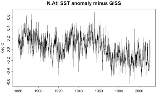
Figure 5: North Atlantic SST minus the global mean.
From a purely technical point, the collinearity introduced between this negative trend in the AMO index and the anthropogenic positive trend confuses the MLR analysis. If you insist on using it, it will give a 50-year anthropogenic trend of 0.1 degree C/decade and a 34-year anthropogenic trend of 0.125 degree C/decade. The 50-year trend is not too much larger than what we obtained previously but these numbers cannot be trusted.
One could suggest, qualitatively, that the negative trend is due to anthropogenic aerosol cooling and the ups and down due to what happens before and after the Clean Air Act etc. But these arguments are similar to the qualitative arguments that some have made about the observed temperature variations as due to solar radiation variations. To make it quantitative we need to put the suggestion into a model and check it against observation. This was done by the HadGEM-ES2 model, and we have discussed above why it has aspects that are inconsistent with observation.
The question of whether one should use the AMO Index as defined by Enfield et al. [2001] or by Trenberth and Shea [2006] was discussed in detail in Enfield and Cid-Serrano [2010] , who argued against the latter index as “throwing the baby out with the bath water”. In effect this is a claim of circular argument. They claimed that this procedure is valid “only if it is known a priori that the Atlantic contribution to the global SST signal is entirely anthropogenic, which of course is not known”. Charges of circular argument have been leveled at those adopting either AMO index in the past, and DumbScientist was not the first. In my opinion, the argument should be a physical one and one based on observational evidence. An argument based on one definition of the index being self-evidently correct is bound to be circular in itself. Physical justification of AMO being mostly natural or anthropogenically forced needs to precede the choice of the index. This was what we did in our PNAS paper.
Enfield and Cid-Serrano [2010] also examined the issue of causality and the previous claim by Elsner [2006] that the global mean temperature multidecadal variation leads the AMO. They found that the confusion was caused by the fact that Elsner used a 1-year lag to annualized data: While the ocean (AMO) might require upwards of a year to adjust to the atmosphere, the atmosphere responds to the ocean in less than a season, essentially undetectable with a 1-year lag. The Granger test with annual data will fail to show the lag of the atmosphere, thus showing the global temperature to be causal.
What is an appropriate regressor/predictor?
There is a concern that the AMO index used in our multiple regression analysis is a temperature response rather than a forcing index. Ideally, all predictors in the analysis should be external forcings, but compromises are routinely made to account for internal variability. The solar forcing index is the solar irradiance measured outside the terrestrial climate system, and so is a suitable predictor. Carbon dioxide forcing is external to the climate system as humans extract fossil fuel and burn it to release the carbon. Volcanic aerosols are released from deep inside the earth into the atmosphere. In the last two examples, the forcing should actually be internal to the terrestrial system, but is considered external to the atmosphere-ocean climate system in a compromise. Further compromise is made in the ENSO “forcing”. ENSO is an internal oscillation of the equatorial Pacific-atmosphere system, but is usually treated as a “forcing” to the global climate system in a compromise. A commonly used ENSO index, the Nino3.4 index, is the mean temperature in a part of the equatorial Pacific that has a strong ENSO variation. It is not too different than the Multivariate ENSO Index used by Foster and Rahmstorf [2011] . It is in principle better to use an index that is not temperature, and so the Southern Oscillation Index (SOI), which is the pressure difference between Tahiti and Darwin, is sometimes used as a predictor for the ENSO temperature response. However, strictly speaking, the SOI is not a predictor of ENSO, but a part of the coupled atmosphere-ocean response that is the ENSO phenomenon. In practice it does not matter much which ENSO index is used because their time series behave similarly. It is in the same spirit that the AMO index, which is a mean of the detrended North Atlantic temperature, is used to predict the global temperature change. It is one step removed from the global mean temperature being analyzed. A better predictor should be the strength of the AMOC, whose variation is thought to be responsible for the AMO. However, measurements deep ocean circulation strength had not been available. Recently Zhang et al. [2011] found that the North Brazil Current (NBC) strength, measured off the coast of Brazil, could be a proxy for the AMOC, and they verified it with a 700-year model run. We could have used NBC as our predictor for the AMO, but that time series is available only for the past 50 years, not long enough for our purpose. They however also found that the NBC variation is coherent with the AMO index. So for our analysis for the past 160 years, we used the AMO index. This is not perfect, but I hope the readers will understand the practical choices being made.
References
Booth, B. B. B., N. J. Dunstone, P. R. Halloran, T. Andrews, and N. Bellouin, 2012: Aerosols implicated as a prime dirver of twentieth-century North Atlantic climate variability. Nature, 484, 228-232.
Chiang, J. C. H., C. Y. Chang, and M. F. Wehner, 2013: Long-term behavior of the Atlantic interhemispheric SST gradient in the CMIP5 historial simulations. J. Climate, submitted.
DelSol, T., M. K. Tippett, and J. Shukla, 2011: A significant component of unforced multidecadal variability in the recent acceleration of global warming. J. Climate, 24, 909-026.
Delworth, T. L. and M. E. Mann, 2000: Observed and simulated multidecadal variability in the Northern Hemisphere. Clim. Dyn., 16, 661-676.
Elsner, J. B., 2006: Evidence in support of the climatic change-Atlantic hurricane hypothesis. Geophys. Research. Lett., 33, doi:10.1029/2006GL026869.
Enfield, D. B. and L. Cid-Serrano, 2010: secular and multidecadal warmings in the North Atlantic and their relationships with major hurricane activity. Int. J. Climatol., 30, 174-184.
Enfield, D. B., A. M. Mestas-Nunez, and P. J. Trimble, 2001: The Atlantic multidecadal oscillation and its relation to rainfall and river flows in the continental U. S. Geophys. Research. Lett., 28, 2077-2080.
Foster, G. and S. Rahmstorf, 2011: Global temperature evolution 1979-2010. Environmental Research Letters, 6, 1-8.
Huang, N. E., Z. Shen, S. R. Long, M. L. C. Wu, H. H. Shih, Q. N. Zheng, N. C. Yen, C. C. Tung, and H. H. Liu, 1998: The empirical mode decomposition and the Hilbert spectrum for nonlinear and non-stationary time series analysis. Proc. R. Soc. London Ser. A-Math. Phys. Eng. Sci., 454, 903-995.
Mann, M. E. and K. Emanuel, 2006: Atlantic hurricane trends linked to climate change. Eos, 87, 233-244.
Trenberth, K. E. and D. J. Shea, 2006: Atlantic hurricanes and natural variability in 2005. Geophys. Research. Lett., 33, doi:10.1029/2006GL026894.
Tung, K. K. and J. Zhou, 2013: Using Data to Attribute Episodes of Warming and Cooling in Instrumental Record. Proc. Natl. Acad. Sci., USA, 110.
Wu, Z. and N. E. Huang, 2009: Ensemble empirical mode decomposition: a noise-assisted data analysis method. Adv. Adapt. Data Anal., 1, 1-14.
Wu, Z., N. E. Huang, S. R. Long, and C. K. Peng, 2007: On the trend, detrending and variability of nonlinear and non-stationary time series. Proc. Natl. Acad. Sci., USA, 104, 14889-14894.
Wu, Z., N. E. Huang, J. M. Wallace, B. Smoliak, and X. Chen, 2011: On the time-varying trend in global-mean surface temperature. Clim. Dyn.
Wunsch, C., 1998: The work done by the wind on the oceanic general circulation. J. Phys. Oceanography, 28, 2332-2340.
Zhang, D., R. Msadeck, M. J. McPhaden, and T. Delworth, 2011: Multidecadal variability of the North Brazil Current and its connection to the Atlantic meridional overtuning circulation. J. Geophys. Res.,, 116, doi:10.1029/2010JC006812.
Zhang, R., T. Delworth, R. Sutton, D. L. R. Hodson, K. W. Dixon, I. M. H. Held, Y., J. Marshall, Y. Ming, R. Msadeck, J. Robson, A. J. Rosati, M. Ting, and G. A. Vecchi, 2013: Have aerosols caused the observed Atlantic Multidecadal Variability? J. Atmos. Sci., 70, doi:10.1175/JAS-D-12-0331.1.


KK Tung: Thanks. The post was easy to read and understand.
Regards
Dr. Tung,
Thank you for taking the time to write this series of posts.
I'm wondering, how sensitive are the results of Zhou and Tung 2013 to the choice of AMO index? i.e. what will the results look like if the index as defined by van Oldenborgh et al. 2009 or Trenberth and Shea 2006 were used instead?
Dr Tung:
The spatial temperature patterns you've shown here are very interesting, but I am concerned that you have attributed a significant amount of temperature variation to the AMO which is already well explained by other causes. In particular I draw your attention to the volcanic record, e.g. here for the recent data, and here for a longer record. The short record is shown below, and shows two clusters of volcanoes with the intervening quiet spells.
The volcanic record explains the apparent oscillation in the temperature record (your figure 4) rather well, with the dips in temperature corresponding to eruptions as follows:
1809-1835: Tambora, Consiguina and two unknown erruptions
1883-1912: Krakatau, Novarupta, Santa Maria
1960-1990: Agung, El Chicon, Pinatubo
This is illustrated by the fit to the data obtained by the Berkeley team using just volcanoes and CO2.
Thank you very much for the posting! I appreciate your effort to elaborate on the AMO issue in such detail. Many points to discuss in much more depth, which I'll do at a later stage (as soon as time allows). For the time being, I would like to clarify and stress that Fig.5 was taken from Tamino! Some may misread that part. It is not mine! While the fluctuations are the true AMO signal (amplifying the external sulfate aerosol forcing), the negative trend is most likely due to the delayed response to the very strong warming once the effect of the Clean Air Act was detectable in the sulfate aerosol loading. It merely reflects the thermal inertia. It's not the aerosols as far as the trend is concerned. The ups and downs are an amplified aerosol response (+ other forcings of course).
As a teaser: I strongly disagree that debate is about whether the observed AMO is anthropogenically forced or not. The debate is about how strong the Atlantic ocean (namely the AMOC) responds to the external forcing. The external (anthropogenic) sulfate forcing is there. We know it! We measured it! It's therefore a well established fact which I won't further discuss. I pointed to the respective literature already. Your reference to the CET time series is therefore rather pointless in my point of view. It just shows how sensitive European climate (and the North Atlantic at that matter) is to external forcing, i.e. volcanic eruptions before the 20th century.
More to come later ...
While it is great to have scientists explaining their published work to the public, I find a little surprising that people still try to do various forms of regression based on surface temperatures and completly neglect the amount of energy going in and out of the ocean - that amount is easily dwarfing the amount of "AMO corrections" and there is a passing mention on how that could be part of the explanation but as far as I can see there is no attempt at including that data into the model and calculations!
Dr. Tung - "The Granger test with annual data will fail to show the lag of the atmosphere, thus showing the global temperature to be causal."
If you examine the correlation of monthly data, as Tamino did here, the AMO has a 2-3 month lag behind global temperatures. It may be that annual data is a bit coarse for this analysis.
I continue to feel that the upward trend of the AMO is an effect, not a cause, of global warming, that the linear AMO detrending retains part of the GW signal and inappropriately removes it in the regression analysis, decreasing the apparent anthropogenic GW signal. The linear detrended AMO is not (as per Trenberth and Shea 2006) an independent variable.
In addition, I would again point to Anderson et al 2012, who find from a strictly energy conservation point of view (ocean heat content versus surface temperatures) that:
[Emphasis added]
Arguments over regression order and detrending aside, there is sufficient evidence to show that the AMO is not capable of causing large portions of recent warming through internal variations (it would have greatly changed the observed OHC values), indicating that results pointing to large AMO contributions suffer from issues.
Reply to post 1 by Bob Tisdale: Thanks!
Reply to post 2 by IanC: Sorry for the late reply; I didn't know my post was finally published online after a long wait, and so I am late catching up with all the good comments.
I mentioned in part 2 the result of using different AMO index, in particular the index by Trenberth and Shea. It is towards the end of that long post.
Reply to post 3 by Kevin C:The relationship between large volcano eruptions and each of the cooling periods for the past 400 years was examined in our PNAS paper. They don't quite line up. Also one needs a series of very large volcano eruptions to have a cooling period that lasts 30 years. Volcanic aerosols do not stay in the stratosphere for more than a year in substantial amount, and ocean inertia may prolong the cooling effect by up to seven years but with diminishing cooling. The time profile is very different than the observed cooling. One can also see in historical data large volcanoes eruptions that did not lead to a cooling period.
Reply to post 6 by KR: By "the upward trend of the AMO" I assume you are referring to the North Atlantic mean SST, because AMO is supposed to be detrended. I agree that anthropogenic forcing can force an upward trend in the N. Atlantic mean SST. In fact I am quite certain of it. In addition I think it is entirely possible that anthropogenic forcing can also force an oscillatory N. Atlantic mean SST. It is just that no credible model has been able to simulate it without contradicting some other aspect of the observation. Furthermore it is difficult to have this theory explain more than two cycles of the observed AMO.
Reply to post 4 by K.a.r.S.t.e.N.: Thank you for pointing out the proper credit of the Figure 5, which I attributed to you.
Currently the debate in peer reviewed literature is about whether the AMO is forced by anthropogenic (tropospheric) aerosol or by the AMOC as a natural oscillation. What you are referring to is a third possibility, that the AMO is forced by the stratospheric aerosol from volcano eruptions. It is possible, though I think it is unlikely ( Please see my comment in post8). But I can be persuaded.
KK Tung @9, I do not think you can say so blithely that the AMO has been "observed". What has been observed is temperature variation in the North Atlantic, and it has been conjectured that that variation is the continuation of a persistent oscillation.
You purport that a persistent AMO has been observed by showing us "Fig 4:, ie, the seventh (and second last) figure in the article above. That compares the fifth Reconstructed Principle Component from MBH98 to the AMO index, and various 50-80 year band signals of various instrumental records. However, the fifth RPC of MBH98 explains only (approx) 3% of the variance of what is, afterall, a NH temperature reconstruction. That low percentate of variance explained almost certainly indicates that the RPC is not significant; and if you are seriously taking it as the AMO signal then you are commiting yourself to the idea that the AMO explains less than 5% of the variance in NH temperatures, an idea I am sure you would reject.
What we have observed in MBH98 RPC 5, then is not the AMO but just some random noise.
What is worse, the actual temperature signal of the CET, which presumably follows that of the North Atlantic very closely, is misrepresented by the "50-80 year band signal" of the CET that you show. This is easily seen in the figure below, which overlays your "figure 4" with the CET temperature series. The blue bars are annual values, while the thin red line is a 21 point binomial smooth of the annual data. It is evident that the "50-80 year band signal" must represent only a small component of the total CET signal; and hence that your "observed" AMO signal is just a small component of North Atlantic temperature variation prior to 1880. If that is the case, either the AMO is not a persistent feature of the NA, or it is a very minor factor in global and NH temperature variation. In either case you have a major problem explaining why it suddenly should appear so dominant in the twentieth century.
In reply to post 11 by Tom Curtis: Most variance of climate data is usually in the high frequencies, and the AMO is in the low frequency. If we judge the significance of a signal by its variance, then one would have arrived at the conclusion that the 100 year long term trend of global warming, which is only 0.8 degrees C, much less than the seasonal, annual, and ENSO variations, must not be significant. Then we would all be wasting our time debating its cause.
The statistical significance of the AMO in the CET data was shown to be at the 95% confidence level, as compared to a red noise model at those frequencies.
In reply to post 3 by Kevin C. El Chichon erupted in 1983, and Pinatubo in 1991, during the most recent period of accelerated warming 1980-2005. This is also the warm phase of the AMO. Volcanic aerosol cools. Tambora, arguably the largest volcano eruption in 300 years, was followed by a warm phase in N. Atlantic. "The year without summer" was only temporary until the ashes were washed out.
Dr. Tung - You are continuing to advocate using a linearly detrended AMO in your calculations, attributing some 40% of warming over the last 50 years to AMO variations.
A linear detrending would be appropriate if and only if warming from other influences over that period were linear. That, however, is not the case. The radiative forcings over that period are distinctly non-linear:
[Source - GISS]
Hence a linear detrending will, as argued by Trenberth and Shea 2006, still contain non-linear portions of that signal, and will inappropriately reduce the global warming signal if subtracted - in effect subtracting a significant portion of overall global warming before attributing temperature changes. As they note:
Linear detrending does not isolate a SST anomaly from overall global warming; a 0.45C misattribution represents roughly 45% of observed warming over the last 50 years - and which matches to the 40% of warming you attribute to the AMO. A linear detrending is therefore inappropriate when attempting to attribute warming against variability.
It may well be (as I believe you have argued) that this becomes an argument of definitions, a chicken/egg question, with different answers based upon the AMO definition. To that extent, it is worth checking assumptions against additional data - for example the Anderson et al 2012 paper I referred to before, and which you have not commented upon. There an analysis of global warming against ocean heat content (OHC) indicates that more than a 10% warming contribution by natural variability is ruled out as inconsistent with observed OHC - if more was contributed by natural variability the oceans would have to be cooler.
The AMO cannot have contributed more than 10% of the warming signal over the last half-century based on conservation of energy, and the 40% attribution you make to the AMO is within 5% of what T&S estimate as misattributed to the AMO by linear detrending. Based on these issues alone, I would have to strongly disagree with your papers conclusions.
KK Tung @12, I would be fascinated to hear what portion of variance in the annual temperature series you ascribe to seasonal temperature differences. Failing that explanation, I have to regard your introduction of seasonal temperature variation when annually resolved temperature differences are the finest resolution under discussion as a pure red herring. Ineed, I also consider the introduction of annual and ENSO variations a case of misdirection when the issue is that your AMO does not show up in the CET series using a 21 point binomial smooth, (described as equivalent to a 10 year moving average by the met office). A 10 year moving average would filter out merely annual variation, along with nearly all variation related to ENSO and the solar cycle. Indeed, if a 50-80 year oscillation does not show up with a 10 year moving average, the most parsimonious explanation is because it does not exist. And it does not show up in the 21 point binomial smooth (equivalent to a 10 year moving average) applied by the MET office to the CET.
Beyond noting your evasions, I note that you have not responded to the first, and key point, that the fifth RPC of MBH98, which you take to represent the AMO, represents around 3% of variance of the NH temperature reconstruction. It is not true for hemispheric temperture records that either the twentieth century warming (or the purported AMO) are much smaller than ENSO or annual variations in temperature. On the contrary, the "hockey stick" in MBH98 comes from RPC1, which explains 38.2% of the variance.
Finally, you are unclear regarding which "AMO" the CET shows statistically significant correlation to. Is it the "AMO" as seen in the 1850- present instrumental temperature set? In that case the lack of an AMO signal in the CET prior to 1850 is strong evidence that there was no such AMO signal prior to 1850. Or was it a correlation with the spurious RPC5? But that RPC is not statistically significant and therefore not a reasonable basis for asserting the existence of an AMO signal prior to 1850.
Replying to post 15 by Tom Curtis: The statistical significance of the AMO mode in the 50-80 year period in the CET data was shown in our PNAS paper.For the global mean data after 1850 it was shown in the appendix of that paper. The statistical significance of the same spectral peak in the multi-proxy data was shown by Delworth and Mann (2000).
Have you tried using longer-term moving average (longer than 10 years)? We did, and it did show up. Moving average is rather primitive and it is difficult to establish the statistical significance of what you generate. We used the wavelet low-pass and band-pass, and there is a well established procedure to establish statistical significance.
Reply to post 14 by KR: How do you know what the total (net) radiative forcing is, given the uncertainty in aerosol forcing?
I did mention in part2 that the effect of removing a nonlinear trend was discussed by Enfield and Cid-Serrano (2010).
Dr. Tung - Uncertainties in aerosol estimates do not mean you can assume extrema values for those aerosol forcings (such as the zero value you seem to use); the most parsimonious estimate is to use the best estimate of that data, as above. Zero is in fact entirely outside the 2-sigma range of aerosol estimates. If you assert that aerosol uncertainties are extreme enough to invalidate radiative forcing data, your own paper has nothing to stand on, as you are attempting to evaluate attribution between internal climate variability and anthropogenic radiative forcings including those aerosols.
Your assumption of linear anthropogenic influence since 1910 is invalid given the totality of observed forcings; which are clearly non-linear in sum. Invoking uncertainty there, however, does not support your work.
Regarding Enfield and Cid-Serrano 2010, I will note a few issues I have with that paper relative to yours:
* They first point out that 1-year lag times are perhaps too long for atmospheric/oceanic interactions, then base their claims of uncertain Granger causality on those 1-year lags. Note that their results are quite ambiguous in this regard, with roughly 50-50% splits depending on test variables and definitions - and that the same test with monthly lag testing indicates a best-fit with AMO lagging temperatures by 3 months.
* They do not support your methods, or a linear detrending, stating "We consider that Trenberth and Shea (2006) and Mann and Emanuel (2006) are quite correct about the desirability of defining the AMO in a way that accounts for the nonlinearity in AGW." I find it curious to see you claiming methodological support from that paper.
* Their detrending, "This can be achieved effectively and simply by subtracting a least squares-fit quadratic function from the time series..." is nearly as simplistic as a linear detrending, and again is not matched to the relevant radiative forcing data.
Finally, as I've noted repeatedly, with no reply on your part, the AMO and oceanic variability simply cannot supply the required energy for 40% of global warming under the energy constraints of rising ocean heat content. Even AMO-driven cloud changes as a possible (if not plausible) secondary mechanism would be insufficient due to their limited duration (they would require forcing changes several times observed) and spatial extent (hemispheric at the very most via teleconnection). Arguing over AMO definitions is a red herring if there is simply not enough energy available to support your conclusions.
I consider this last issue just as important as the AMO definitions - the influence of internal variability must be consistent with all the available evidence.
---
Enfield and Cid-Serrano 2010 does not support linear detrending, uncertainties in aerosols can only weaken your own conclusions, and you have not addressed the energy balance issue in any way. I'm afraid I must continue to disagree with your conclusions.
Reply to post 18 by KR: I did not assume that aerosol forcing is zero. I in fact think they are slightly larger than what has been used in GISS models, with the difference well within the range of uncertainty for tropospheric aerosols.
KK Tung @16, here are the 10, 15 and 20 year running means of the CET from 1660 to 2012:
As you can see, there is no consistent 50-80 year oscilation in the data. There is what might be a large amplitude 80 year oscillation from 1660-1740. However, the trough of that "cycle" corresponds with the Maunder Minimum and a large number of large volcanic erruptions, while the peak corresponds to a period without significant volcanic activity. In other words, that "oscillation" is more likely a result of forcing than not. Then from 1740 to 1910 there are seven distinct peaks indicating average "cycle" lengths of 25 years, although the cycles vary in both magnitude and length. The longest cycle length (treating the smallest peak as an aberration) is less than fifty years in length. Finally, from 1910 to 2012 you may have two cycles of 50 plus years. There is certainly no consistent periodicity over the entire period.
Tellingly, this pattern (or lack of it) shows up in your supplementary material, and specifically in figure S2:
Clearly the 50-90 year signal is almost entirely absent from about 1750 to about 1910. In contrast, during that period there is a strong 32 to 50 year signal. There is simply no compelling reason to consider the 50-90 year bandwidth a representing a physically important process while relegating the 32-50 year signal to irrelevance; and if we allow ourselve so broad a target as an oscillation that varies by a factor of 2-3 in amplitude and by more than a factor of 3 in period, it becomes almost impossible to not find your AMO in any random data.
Speaking of which, you claim a statistically significant 50-80 year AMO over the full length of the the CET record based on a wavelet analysis. Tamino has some very interesting comments on such analyses. Specifically, standard significance tests applied to wavelet analysis will overstate the statistical significance of observed oscillations because they do not allow for the fact that we are searching a large range of hypotheses simultaneously. To the extent that you have not compensated for that, therefore, your wavelet analysis will also overstate the statistical significance of the "detected" AMO signal.
I think KR's comments on use of all the forcings is critical. In particular, I think that this key comment from your article is overstated:
In fact, Hansen's model at least comes very close if you take into account internal variability in the for of El Nino. I haven't looked at the others, but here is a result from a simple 2-box model illustrating this fact:
This trivially simple model is available here for you to play with - for the figure above, just click 'Calculate'.
The key to this model is that it takes into account both forced response and ENSO. If you leave out the ENSO term (figure 5 on that page), then the model appears to fail to reproduce the mid-century cooling. When including it (figure 1) the model fit is extremely good except for 2 spikes either side of WWII. The temperature record is GISTEMP and so is missing the post-war SST adjustments, which probably accounts for much of the remaining discrepancy.
The significance of the ENSO term is that the trend in MEI on the period 1940-1960 is about 70% of the trend on 1997-2013. ENSO plays a significant role in the cooling on that period, and of course only corresponds to a single realisation of climate variablility. Using an ensemble of runs or alternatively using a simple energy balance model allows us to eliminate the internal variability. Imposing the real ENSO contribution allows us to figure in the actual realisation. The resulting model fits 92% of the variance in the data. You can test the skill by omitting different periods from the model fit.
We could redo the calculation with Hansen's data instead of the 2-box model, but the results will be similar. Ideally we'd use a longer time frame too. BEST should be significantly better than CET, and the Potsdam forcing data goes back to 1800 (although I think it omits the 2nd AIE). I'm afraid I haven't had a change to do this calculation yet.
Kevin, impressive comparison. Is there some more info somewhere on the ins and outs of the model and analyses used? In particular, is it using the Green's function of GISS model-E?
Dr. Tung - If you are including the aerosol forcings and their changes over time, the sum forcings are again not linear since 1910, as per the figure in my post above. Note that not only tropospheric but stratospheric aerosols are involved in the "S" curve seen in 20th century forcing data. There is simply no support for a linear forcing during the 20th century, a requirement for your claim of a linear warming since 1910.
As per Kevin Cs comment, and your claim that "no CMIP3 or CMIP5 models have successfully simulated the observed multidecadal variability in the 20th century using forced response", I would simply point out Figure 9.5 from the IPCC AR4 report:
Figure 9.5. Comparison between global mean surface temperature anomalies (°C) from observations (black) and AOGCM simulations forced with (a) both anthropogenic and natural forcings and (b) natural forcings only...
Note that the models using all forcings match multi-decadal temperature variations quite well, including a mid-century pause. I fail to see significant support for your statement.
Bart: No, it's the 2-box model of Rypdal 2012 with an extra ENSO term - the response function is determined by fitting the forced response to the data. However the forced response is similar on the decadal level to the temperatures obtained by Hansen 2011 using the Green's function mode. The only difference is that he uses the model to get the response function.
Tamino writes about his version here.
You can actually get a marginally better AIC using 1.5 boxes (1-box + transient).
In reply to post 23 by KR: Figure 9.5 from AR4 is the figure that I often used to show that while the warming since midcentury has been simulated quite well, the early twentieth century warming has not been simulated. Compare the slope of the red curve with the slope of the black curve. So far only HadGEM-ES has simulated the early twentieth century warming using forced solution by varying tropospheric aerosols, but it has other problems mentioned by zhang et al 2013.
In reply to post 20 by Tom Curtis: We had discussed in our paper why we chose the band 50-90 years and exclude the band around 40 years. This was based on comparison with the global mean spectrum. We believe the 40 year oscillation, while also a part of the AMO, does not have a global manifestation. That is, it may have affected Atlantic and Europe, but not the Pacific. During the middle cycle in the 1700s 1800s, the AMO's period switched to 40 years and only part of it remained in the 50-90 year part.
No one is referring to the AMO as a sinusoidal oscillation with an unchanging amplitude and period. It is only quasi-periodic.
[Sph] Date corrected as per KK Tung's later comment.
KK Tung @26:
1) The caption of Fig 3B of the PNAS paper (ie, the "Fig 4" above) reads:
The periods of 50 to 90 year band signal of the multiproxy data (MBH 98 RPC5) from peak to peak are approximately, 72 years, 70 years, 110 years and 76 years. There is no hint of the AMO switching to a 40 year period in the 1700s. Now, if the AMO period switched to 40 years in 1700s, and there are no 40 year cycles in the multiproxy AMO signal, they do not agree "in phase" and the appearance that they do so is only a product of your filtering. Hence, you cannot consistently claim both that the CET signal reflects the AMO in the 1700s and that MBH 98 RPC 5 is the AMO signal.
That inconsistency leaves you with a small problem. If you decide (reasonably given its low statistical significance) that MBH98 RPC 5 is not the AMO signal, then you are left struggling to explain why the AMO cannot be dectected in multi-proxy NH temperature reconstructions despite its purportedly dominating influence on NH temperatures in the twentieth century. If, instead you decide to use MBH98 RPC5 as your AMO signal, your are left struggling to explain its low variance explained and why the AMO was so uninfluential CET temperatures over much of the historical period.
2) Allowing that the AMO switched to very short periods (around 25 years in the mid 1700s), you need to explain why the AMO appears only to have high amplitudes and an extended period durring periods of significant forcing (Maunder Minimum, 20th century). Absent that explanation, the most conservative conclusion is that the extended AMO is a response to that forcing, either directly or indirectly. In that case, the AMO may complicate the timing of the response to forcing, but is not an independant factor.
3) I regard with extreme skepticism such humpty-dumpty oscillations whose periods can be stretched like taffy to suit the convenience of the theoretician. In science it is not a question of "which is to be master" but of what is observed. More specifically, the theory of the AMO is that a quasi periodic oscillation exists in the Atlantic with a period of about 65 years. Once that period can be stretched like taffy to fit any observation, you are merely defining the AMO into existence, not observing it.
4) Even if you present us with a theoretical justification for so extraordinarilly flexible an oscillation, which you have not, the mere fact of its fexibility reduces its the possibility of detecting it in that for a very flexible period (and amplitude) almost any observation can be made to fit the theory. In short, I think your theory of the AMO has become unfalsifiable and hence devoid of empirical content.
Kevin C @ 21,
That is really very cool. I'm particularly intrigued by the fact that you can actually get a very good fit for the entire series using just the years 1880-1950 (R2 = 0.714) even without the post-WWII SST corrections in the temperature data.
I'd say that "key comment from your article is overstated" is an understatement. :-)
Also intriguing is that the improvement of the qualify of the fit in the last few decades has come as a result of increasing TCR:
I presume that the change in TCR isn't statistically significant, due to the accuracy of the early data especially, but the fact that numerically it gets larger when we add the decade where warming supposedly "stalled" is telling...
Jason: Yes, we're discussing it here.
Dr. Tung - The comparison of models to observations show that observations are within the 2-sigma range of those models. That's not a failure of the models, but rather an indication of their success, even though the model mean averages out ENSO variations across the models.
Models that are fit to forcings and to observed ENSO variations, such as the one Kevin C pointed out, are much closer fits to the data.
---
The linear detrending of the AMO used in your paper is wholly inappropriate for attribution studies, as is noted by one of the very papers you rely on for your argument (Enfield and Cid-Serrano 2010). Forcings over the last century are non-linear, and a linear detrend leaves much of the warming signal in the AMO component, causing an underestimation of global warming as in your paper. Your assumption of linear warming is therefore a circular argument. Your cycle identification, and use of the CET, has other issues of non-periodicity as noted by Tom Curtis. And you have continued to completely ignore the energy balances (Anderson et al 2012, and for that matter Levitus et al 2001, Levitus et al 2005, and other works) that show the AMO and other internal variation cannot be contributing significantly to global warming given observed ocean heat content.
You have not, in my opinion, made your case, and I would continue to agree with the analysis first raised here - that your conclusions regarding a low warming trend are unsupported.
Dr Tung wrote "Figure 9.5 from AR4 is the figure that I often used to show that while the warming since midcentury has been simulated quite well, the early twentieth century warming has not been simulated"
Like KR, I find this a rather odd statement. The multi-model mean is not directly a prediction/hindcast of GMST, but only of the forced component of the change in GMST. As such there is absolutely no reason to expect the observed GMST to lie any closer to the multi-model mean than within the spread of the model runs (as the spread is implicitly an estimate of the plausible magnitude of the unforced response). The figure shows that the models give as good a hindcast of 20th century temperature variations as we could reasonably expect, given what the models are actually intended to achieve.
Even if the model physics were exactly perfect, the observation would still be expected to lie only within the spread of the model runs, and there would be absolutely no reason to expect them to be any closer.
So the question I would like Dr Tung to answer is "Exactly how close to the multi-model mean would you expect the observations to lie in order to give a good hindcast of 20th century temperatures, and how would you justify this estimate of the magnitude of the unforced component?".
On second reading, Dr Tung wrote "Compare the slope of the red curve with the slope of the black curve." They look rather similar to me, provided you aren't looking at decadal variation, which is largely due to unforced variability (e.g. ENSO) which is deliberately averaged out in computing the multi-model mean (as the "ENSO" in individual model runs can't reasonably be expected to be synchronised with the observed ENSO, as ENSO is a chaotic phenomenon).
It seems to me that the purpose of computing the multi-model mean is not well understood in discussions of climate, but the bottom line is that it is not a prediction/hindcast of the observed climate change, just a prediction/estimate of the effects of the forcing on the climate. These are not at all the same thing!
From Page 595 of the IPCC AR4:
8.1.2.3 Testing Models Against Past and Present Climate
...
Differences between model and observations should be
considered insignificant if they are within:
Note in particular, item 1. If someone wants to show that the model hindcast is poor, they need to be able to show that the error exceeded the uncertainty due to internal variability.
In reply to post 31: "So the question I would like Dr Tung to answer is "Exactly how close to the multi-model mean would you expect the observations to lie in order to give a good hindcast of 20th century temperatures, and how would you justify this estimate of the magnitude of the unforced component?""
The ensemble mean, especially multi-model ensemble mean, should reveal only the forced response. The difference should be accounted for by the unforced variability (if we assume that the models' forced response is correct). Although there is quite a bit of inter-model scatter, about 0.3 C, as often happens when you have an ensemble of different models with different levels of quality, one can see in AR4's Figure 9.5 a difference in slope between the red curve and the black curve. I hear what some of you are saying about the fact that the difference still lies within the scatter, and therefore there is no need for an unforced variability and that the AR4 models are doing well simulating the historical data in the early twentieth century as well. As a scientist we pay special attention to the systematic discrepancies between model and observation, and I see a systematic underprediction of the observed warming rate in the early part of the twentieth century by the CMIP3 models. This just my opinion. You do not need to agree with me on this.
Correction to my post 26: 1700s should be 1800s.
[Sph] Original comment revised to help avoid confusion.
Dr. Tung - Given the large number of La Nina events from ~1915-1935, followed by a decade long El Nino state centered around 1940, the first qualification of the IPCC report should apply:
[Source]
I believe that unusual run of ENSO is a more than adequate reason for a slightly higher slope than non-ENSO modelling in the beginning of the 20th century - without invoking huge internal variations inconsistent with ocean heat content. I consider your claims of poor focing/climate modelling in the early 20th century unfounded.
Interesting graph KR. I note too though there is an unually large no. of EN events from 1975 to 2000 which would imply observed warming about background levels.
scaddenp - Indeed, which makes the 2000-2012 "slowdown" accompanied by more of a balanced ENSO distribution (ending in significant La Ninas) far more understandable; the expected effects of short term variations against recent history.
KK Tung @34: " As a scientist we pay special attention to the systematic discrepancies between model and observation, and I see a systematic underprediction of the observed warming rate in the early part of the twentieth century by the CMIP3 models. "
[Refering to the graph presented by KR @23]
Other than your eye, what basis do you have to say that it is a systematic underprediction? Exactly how are you determining which part of the observations represent systematic behaviour, and which part represent random behaviour? (Note that I am asking a somewhat rhetorical question: from what I've read in the posts and your comments, my impression is that you have determined that the observations have systematic behaviour because you've assumed that the behaviour you see is systematic.)
GCM simulations, by their nature, will have random variations over time, if you start them from slightly different initial conditions. Each simulation represents a realistic sequence, but any one of them will be possible. The observations only represent one sequence. It's like rolling dice: you can have one sequence of numbers originating from rolling the dice 100 times, and a computer model "throwing" dice via a random number generator. When you compare the two, you don't expect an exact match. Doing 20 computer simulations and averaging them will give a sequence closer to the middle, but the observations can still fall anywhere in the expected range for a single sequence. (The analogy isn't the best - rolling dice is purely random, with no systematic pattern in the trend over time.)
It is simply a mistake to think that the ensemble model mean is what nature is supposed to do: even with a perfect model, nature could follow any one of a large number of different sequences from the model. The correct thing to do, if the observations fall wihtin the range of the individual model runs, is to accept that there is little else you can say about the comparison.
You simply can't expect the non-stochastic behaviour of the model (average of a number of runs) to follow the stochastic nature of a single run (or observations). If you try to do so by adjusting the model, you are fitting to the noise. In such a case, fitting to a different sequence (e.g., a different time period) with different noise will require different adjustments to the model - and it won't mean anything because the underlying physics is still the same and you've just taken noise and interpreted it as signal.
...which appears to be exactly what you are doing with your study: you have mistaken noise for signal, and see a pattern that you think means something, but the pattern is just an artifact of the particular sequence of noise in the data.
I, like others here, remain unconvinced.
KR @36, the cool aberation from 1907-1914 at least partially overlaps the strong El Nino event starting in 1910, and hence is not entirely explained by ENSO. Likewise the warm aberation from 1937-1946 is longer, and starts earlier than the major El Nino of 1940-1943. (Dates determined by eye so not exact.) Consequently while ENSO may partially explain these aberations, there remains something to be explained once we have accounted for ENSO. I personally am inclined to think that Black Carbon forcing durring the war years has been underestimated, but obvoiously that is just a guess.
KK Tung @34, here is Fig 9.5 A of AR4 overlaid with HadCRUT4 running 12 month mean along with the trends from 1900-1960 and 1910-1940:
Clearly both trends are greater than that of the multimodel mean over equivalent periods. That being said, the 1900-1960 trend clearly lies above the data from 1945 on, suggesting that it has been dragged up by the 1937-1946 temperature excursion. It is fair to say, therefore, that the multimodel mean accurately predicts temperatures in the early and mid twentieth century except from 1937 to 1946. Given that the world was in a state of war durring that period (remembering not just WW2, but Spain, Manchuria and the Sino-Japanese wars) it is at least plausible that the excursion is either an artifact of reduced temperature measurements or the result of unusual and as yet undetermined forcings resulting from the devestation of modern warfare.
Of course, if the appropriate trend comparison is 1910-1940, such possibilities will be inadequate to explain the discrepancy. However, for 1910-1940 to be the appropriate period of analysis, we need an independent reason for distinguishing that period. Without that independent reason, focusing on an interval starting with an unusual low and ending with an unusual high in tempertures is just another game of cherry picking.
You will argue, no doubt, that the existence of the AMO give sufficient reason to focus on that interval. I would disagree. You have not established the existence of an AMO prior to the twentieth century, and your reason to consider the twenteith century AMO independent from known forcings comes down, in the end to the 1940s temperature discrepancy. Consequently, the is not evidence of a globaly influental AMO, but only that something occurred in the 1940s which is not yet adequately explained. The AMO is one candidate explanation among others. Indeed, the lack of a regular, influental AMO prior to the twentieth century makes it, IMO, a very weak alternative explanation. So weak that it is in danger of being merely ad hoc.
Tom Curtis - Quite right, dates (and variability) are not exact. Just keep in mind that while the ENSO represents a major portion of the climate variability, it doesn't cover all of it. However, the 1915-1935 La Nina's and the 1935-1945 El Nino have a significant effect on short term temperature slope over that range.
I would not at all be surprised by significant black carbon influences - without satellite measures in the WWII period, it would be difficult to say how much BC was present due to basic fire effects during war years. To estimate that would require extrapolating war damage to black carbon production, and I am not aware of any work in that respect.
Does anyone know of relevant papers?
Tom Curtis - Also worth noting are data discrepancies during the war years, and during the change-over from bucket/engine-room/buoy measures of ocean temperatures. I'm not convinced that all of those data issues for the 1940's have been resolved.
Dear Prof Tung,
thank you for this impressive posting and the valuable comments. As you mentioned Rahmstorf/Forster, I think their paper failed due of the assumption that the ENSO index is linear to the global temperature effect of the ENSO process. Such linearity is a basic prerequisite of a linear regression. The reason for the non-linearity is mainly due to El Nino warm water pools drifting out of the ENSO index region and continuing to warm for years, though no longer measured by the ENSO index. Detrended AMO appears to be the better choice, PDO may be another good choice IMHO.
Dr Tung I'm sorry, but you have not answered my question. It may be your opinion that there is a systematic underprediction by the CMIP3 models, but if you want others to agree with your opinion you need to be able to provide adequate justification for that opinion.
As scientists (I am also a scientist) we do indeed pay special attention to the systematic discrepancies between model and observation; however as scientists we should not stop at observing a visual discrepancy. The human eye is rather too good at seeing "systematic features" in signals where in reality there is only noise, which is why we have statistics to provide an objective test for our hypotheses (even if only a sanity check). So at the very least, a scientist should determine whether there is adequate evidence that the apparent discrepancy actually is systematic, rather than being merely an artefact of the noise (in this case internal unforced climate change). My question was intended to help you to explain the evidence for a systematic discrepancy, and so far you have provided none. I still have an open mind on this, but I require evidence.
Note I wouldn't go as far as to say that the models give good hindcasts of 20th century climate (in absolute terms), just that their hindcasts are as accurate as we have reason to expect. If someone can show that the plausible magnitude of the effects of unforced internal variability is substantially smaller than the spread of the model runs, then there may be an argument that the accuracy of the hindcasts falls below that we could reasonably expect. The problem is that we have only one realisation of the observed climate, with ever changing forcings, so it is difficult to see how we can estimate the magnitude of unforced internal variability without using models in much the way they are currently used.
At the end of the day, there needs to be an element of self-skepticism in good science, in this case, the null hypothesis should be that the apparent discrepancy is due to internal variability and the onus is on yourself to demonstrate that this is implausible, as it is your claim that a systematic discrepancy exists. That is conventional scientific practice.
MS1 "I think their paper failed " really? The paper investigated how much of the variability of the temperature record could be accounted from assuming simple relationship with 3 known causes of internal variability. Rypdal 2012 showed it could be improved but F&R is remarkable successful. Tests with only using part of the data for training show it also a robust predictor of future variability.
If the ENSO index was substantially flawed or there was significant non-linearity, this isnt born out by the success of their prediction. If you believe that the prediction can be improved significantly by other indexes or method, then show us.
KK Tung @10:
I am referring to forcing from tropospheric (anthropogenic) and stratospheric (volcanic) aerosols likewise. They have an impact on both, the AMOC and the AMO. Sure, the response of the AMOC to external forcing is slower and hence harder to identify, but neither AMOC nor AMO are independent of it. I agree that the AMO is influenced by the AMOC (how can it not). The exact linkage is still under debate. However, I strongly disagree with your reply to Kevin C in post 8 and your notion that a volcanic impact on the AMO is unlikely. Let me try to convince you.
In your paper, you wrote: “The 20-y small dip in temperature near 1810 coincides with the solar Dalton Minimum, but is probably caused by a negative excursion of the AMO. The rising AMO cycle in the first half of the 19th century produced a warming, despite the eruption of Tambora (1815), the largest in the past four centuries.”
The problem is that we have a strong volcanic eruption in 1809 (unknown tropical eruption; see Cole-Dai et al. 2009 or Arfeuille et al. 2013), followed by the 1815 Tambora eruption (strongest eruption in the last centuries). Hence I have no doubt whatsoever as to what the reason of the negative AMO excursion is. It’s entirely attributable to these two strong eruptions. The surface air temperature over the Atlantic-Arctic boundary in your Fig.3C perfectly matches the timing of these eruptions. If we go on to the 1830s, we see the next dip which perfectly matches with the Babuyan Claro eruption (1831) and the next very strong eruption at Cosiguina in 1835. The dip around 1860 is stronger than one would expect from the amplitude of the corresponding eruption recorded in 1861, only to have a clear signal for the Krakatau eruption in 1883 again. Note that the exact magnitude of the volcanic forcing differs between different estimates. I plotted the older dust veil index (DVI) and the newer ice core index (ICI) from Crowley and Unterman 2012 for the time period 1750-2000 in order to illustrate my point.
Moreover, I consider it very likely that volcanic eruptions do have a measurable effect also on the AMOC. Gleckler et al. 2006 and Stenchikov et al. 2009 demonstrate that a persistent deep ocean signal emerges after strong volcanic eruptions. Therefore, most of the time the climate system is not in an equilibrium state as it takes several centuries to get rid of any remaining signal from volcanic eruptions. As soon as there is a lull in volcanic activity, the climate system warms in order to restore equilibrium. I don’t know how strong this warming signal is, but it definitely plays a role in post-volcanic periods such as that between 1910-1940. I agree with Tom Curtis (post 40), that this period saw some additional warming in the North Atlantic region due to increasing black carbon forcing (while anthropogenic sulfate forcing was barely rising during that very time). The external forcing impact on the AMOC is also widely discussed in the literature, with numerous suggestions as to what mechanisms could be at play. I would like to point at a very recent paper by Menary et al. 2013 or another one by Iwi et al. 2012. It goes without saying that undoubtedly internal AMOC variability exists undoubtedly. The review paper by Kuhlbrodt et al. 2007 gave a good overview.
Similar to what Kevin C did (see post 21), I recently developed my own two-box EBM model which accounts for volcanic eruptions at two time-scales: A fast surface temperature response which more or less coincides with the stratospheric AOD evolution, and a slow response which accounts for the deep-ocean signal as shown for the Tambora and the Pinatubo eruptions in Stenchikov et al. 2009. In addition, instead of using the GISS forcing (which I personally consider not very accurate regarding the tropospheric aerosol forcing) I used the forcing time series for sulfate and black carbon aerosols presented in Skeie et al. 2011. The resulting forcing function (nudged towards NH conditions) for the 1750-2010 period looks like this (I can provide more details upon request):
Not only are the volcanic spikes easy to identify, but also becomes their long-term effect noticeable. I am not claiming that this is the real volcanic fingerprint which we find in the observations, but it indicates where we might have to look for a forced disturbance in the thermohaline circulation, may it be the AMOC or ENSO/PDO. Let’s compare the forcing function with the NH instrumental observations and reconstructions:
Note that the temperature response in Europe as represented by the Berkeley Best data and Baur temperature series (both are comparable with the AMO temperature trends) is not always in phase with the rest of the NH. In fact, there is reason to think that the NAO response to volcanic eruptions is preferably positive. Fischer et al. 2007 have a good discussion on that. Assuming that the NAO and the AMO mutually influence each other, stochastic multi-annual or decadal variations as a result are all but surprising. Even in the absence of NAO-like atmospheric variability, Deser et al. 2010 brilliantly illustrate how white noise from pure random atmospheric heat flux variations turns into (oceanic) red noise. The time scale of the resulting SST fluctuations depends on the ocean mixed-layer height. It is interesting to note that the mixed-layer depth of the North Atlantic is comparably high, particularly in winter, which can easily explain the high standard deviation of its SSTs. The same is true for large portions of the North Pacific.
This brings me to DelSole et al. 2011, which you cited in your response. Likewise, they identified these very regions as most variable. However, I can’t see how the “projection” of the observed temperatures onto this pattern removes the problem of unreliable model forcing. As can be seen from my best-guess forcing assumption for the NH (which includes aerosol indirect effects, which most models omit altogether), the real forcing has likely been considerably more variable than assumed in your analysis as well as in their analysis (which is based in the forcings of the models used). This can also be illustrated by looking at the NH/SH inter-hemispheric temperature trend. Not only does it differ considerably, but also is the NH instrumental record strongly correlated with the anthropogenic sulfur emissions, which is almost certainly not a mystic coincidence.
Many other issues regarding the robustness of your results have been raised in the discussion already. I agree with Tom Curtis (post 11/15) on the magnitude of the AMO signal in the NH temperature variance, which I believe your method terribly deflates, as well as on the consistency and significance of the oscillation in the data (post 15/20), which I believe you have not demonstrated. Conservation of energy is another is another big problem (see e.g. KR in post 14) which you have so far failed to address properly.
Finally, let me show you what happens if we extend the forcing time series back in time and keep comparing it with paleo-reconstructions. With a low-pass filter it looks like this:
From a NH point of view, the AMO plays a minor role as far as the temperature evolution is concerned. Not to mention global temperatures. The AMOC is important on longer time scales, typically in response to slow changes in external forcing. On shorter time-scales, AMOC changes can have strong regional impacts. The AMOC shutdown in the context of the 8.2ka event as the prime example for its response to strong fresh water pulses.
I am trying to catch up with the replies after a busy week.
Some of the comments concern my statement that I thought there was a systematic underprediction of the observed rate of warming in the early twentieth century by the CMIP3 models. Opinions were expressed that statistically they agree within two standard deviations of the model spread. That model spread is rather large. If you are satisfied with that, that is fine with me. To me I see that the multimodel mean produced only 50% of the observed warming during the first half of the 20th century. Our proposal was that that 50% was caused by an internal variability (viz the AMO). We do not expect the ensemble mean to contain this internal variability. And I am not sure how the models can be made to do it since we do not know the initial condition in the ocean sublayer well in 1850-1870 (the time these model simulations start).
I agree entirely with Bob Loblaw in post 39. The observed climate is one realization of many possible climates. It is important to point out that one realization should in principle contain a particular phase and amplitude of the AMOC, an internal variability. There was a warm phase in the first half of the twentieth century. It is not reasonable to expect the model ensemble to produce it. Also, even if we use a single model realization, that realization may contain a different AMOC phase. My comments about the CMIP3 model underpredicting the warming should not be taken as a criticism of the models; they are expected to robustly generate only the forced solution. But the point remains that there is another part that is important but was not simulated.
One could take the point of view that the internal variability is just climate noise, and that the difference from any such unpredictable (by models) internal variability should be considered as "insignificant" (p595 of AR4) (post 33 here). This is in essence a statement that we will ignore internal variabilities just because we have not found a way to simulate it using the current generation of models.
Looking into this subject a bit further, I would like to point out Ting et al 2009, Forced and Internal Twentieth-Century SST Trends in the North Atlantic as a recent work that summarizes a great deal.
This paper examines the various components in the AMO using Empirical Orthogonal Function (EOF) analysis, which is a principal components analysis including both time and spatial patterns. They find that EOF analysis supports detrending North Atlantic sea surface temperatures using either global sea surface temperatures (SSTs) or global mean temperature, not a linear detrending, as linear detrending aliases external forcing into the AMO index.
FIG. 2. (a) The linear trend (solid black line) and detrended NASSTI (shaded). (b) NASSTI regressed onto the global mean SST (SSTg regression, solid black line) and the difference between the observed NASSTI shown in Fig. 1 and the SSTg regression (shaded). (c) NASSTI regressed onto the global mean surface temperature (Tg regression, solid black line) and the difference between the observed NASSTI shown in Fig. 1 and the Tg regression (shaded).
This supports works such as Trenberth and Shea 2006, with rather more numeric backing; the first EOF component dominating:
Note that the mid-century AMO is supported as a real, internal variation - but at end of the 20th century a linear detrended AMO is heavily aliasing global warming. This indicates that, rather than the AMO presently being at a peak influence and perhaps about to decline, it instead has the possibility of rising over the next few decades increasing North Atlantic temperatures above that driven by external forcings - whether the AMO increases or reverses in the near future will have a significant effect on Atlantic region temperatures. And the late 20th century AMO influence is actually quite small.
I would be very interested in what external forcing vs. internal variation analysis would conclude regressing against a more accurate AMO index. But I repeat that a linear detrending is inappropriate, aliases the global warming signal, and (in context with respect to the Tung et al paper) linear detrending leads to a significant underestimation of external forcings.
This has been a most interesting, truly scientific debate, all too rare on blogs. I can think only of RC as another place where such discussions could happen .Not surprisingly, there is no noise about it in the denialosphere.
I understood a couple of years ago that this was the direction where SkS was heading and thus stepped down as a moderator, as I did not have the time to participate at that level, nor to qualify myself in order to do so. I think KR is pretty close to the point where he could put together his own paper. Not to put pressure on anybody :-) but it would certainly be a useful elaboration on Dr Tung's published work and in the interest of continued scientific debate and fostered understanding...